Sorting Algorithm A Summary

#

Introduction

#

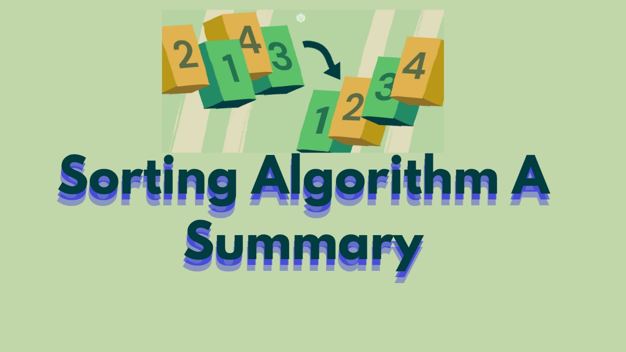
Sorting is a fundamental operation in computer science and plays a vital role in various applications. Whether it’s organizing data, searching for specific elements efficiently, or preparing data for further processing, sorting algorithms provide the necessary tools to bring order to chaos. With a wide range of sorting techniques available, each with its own strengths and weaknesses, it is essential to understand their principles, time complexities, and trade-offs.

In this comprehensive guide to sorting algorithms, we will explore a variety of popular and essential sorting techniques. We will delve into their inner workings, discussing the key ideas behind each algorithm and explaining their step-by-step processes. Additionally, we will examine the time and space complexities of each algorithm, helping you evaluate their performance characteristics and choose the most suitable approach for specific scenarios.

By the end of this article, you will have gained a comprehensive understanding of a wide range of sorting algorithms, empowering you to analyze and select the optimal sorting technique based on your requirements. Whether you are a student exploring computer science concepts, a software developer seeking efficient sorting solutions, or simply someone curious about the inner workings of algorithms, this article will serve as a valuable resource on the fascinating world of sorting.

Important Sorting Algorithms

#

• Bubble Sort: Repeatedly compares adjacent elements and swaps them if they are in the wrong order. The largest (or smallest) element “bubbles” to the end (or beginning) of the array in each pass.

• Selection Sort: Finds the minimum (or maximum) element in the unsorted part of the array and places it at the beginning (or end) of the sorted part. It iterates through the array, selecting the smallest (or largest) element and swapping it with the appropriate position.

• Insertion Sort: Builds the final sorted array one element at a time by repeatedly taking an element and inserting it into its correct position in the sorted part of the array.

• Merge Sort: Divides the array into two halves, recursively sorts each half, and then merges the two sorted halves to obtain the final sorted array. It uses the divide-and-conquer approach.

• Quick Sort: Selects a pivot element, partitions the array into two parts (elements less than or equal to the pivot and elements greater than the pivot), and recursively applies the same process to the two partitions. It also uses the divide-and-conquer approach.

• Heap Sort: Builds a binary heap from the array and repeatedly extracts the maximum (or minimum) element, placing it at the end of the sorted array. It uses the heap data structure to perform the sorting.

• Radix Sort: Sorts elements by processing individual digits or characters. It works by distributing the elements into buckets based on the value of a specific digit and repeatedly redistributing them until all digits have been considered.

• Counting Sort: Sorts elements based on their frequencies. It counts the occurrences of each element in the input array and uses this information to determine the position of each element in the sorted array.

• Bucket Sort: Divides the range of input values into a set of buckets, distributes the elements into these buckets, and then sorts each bucket individually. It is useful when the input values are uniformly distributed.

• Shell Sort: A variation of insertion sort that starts by sorting elements that are far apart and progressively reduces the gap between elements. It combines elements of insertion sort and bubble sort.

• Tim Sort: A hybrid sorting algorithm derived from merge sort and insertion sort. It performs a combination of insertion sort and merge sort to achieve efficient sorting, particularly for real-world data sets with natural ordering.

• Comb Sort: A variation of bubble sort that compares elements that are a certain distance apart and swaps them if necessary. The distance between elements gradually decreases with each pass, similar to the shrinkage of a comb’s teeth.

• Pigeonhole Sort: Suitable for sorting elements where the number of distinct values is not significantly greater than the number of elements. It places each element into its corresponding pigeonhole and then retrieves the sorted elements from the pigeonholes.

How Sorting Algorithm Works.

#

For understanding the working of all four important algorithms we will take following array:
Array = [9, 5, 89, 1, 4, 77, 3, 9]

How Merge Sorting Works:

#

• Divide: Divide the array into two equal-sized subarrays.
• Conquer: Recursively divide and sort.
• Merge: Merge all the subarrays.

Array = [9, 5, 89, 1, 4, 77, 3, 9*]
Divide 1:
Subarray 1: [9, 5, 89, 1]
Subarray 2: [4, 77, 3, 9]

Divide 2:
Subarray 1.1: [9, 5] => [5,9]
Subarray 1.2: [89, 1] => [1,89]
Merge1: [1,5,9,89]

Subarray 2.1: [4, 77,] => [4, 77]
Subarray 2.2: [3, 9] => [3,9]
Merge2: [3,4,9,77]

Final Merge:
[1,3,4,5,9,9,77,89]

How Quick Sorting Works:

#

• Select: Select a pivot element from the array. In this example, we’ll choose the last element, 9, as the pivot.
• Partition: Rearrange the array so that all elements smaller than the pivot are placed before it, and all elements greater than the pivot are placed after it.
• Recurssion: on the subarray

Array = [9, 5, 89, 1, 4, 77, 3, 9*]
Itr1: [5, 1, 4, 3, *9, 77, 89, 9]
subarray: [5, 1, 4, *3], [9, 77, 89, *9]

Itr2:[1, 3*, 5, 4], [*9, 9, 77, 89]
Subarry: [1,3], [5,4], [9, 9], [77, 89]

Itr3: [1,3], [4,5], [9, 9], [77, 89]

Final: [1,3,4,5,9,9,77,89]

##Selection sorting : It works by repeatedly finding the minimum element from the unsorted part of the array and placing it at the end of the sorted part. Select a pivot element from the array. In this example, we’ll choose the last element, 9, as the pivot.

Array = [9, 5, 89, 1, 4, 77, 3, 9]
Sorted Part : Unsorted Part
[] : [9, 5, 89, 1, 4, 77, 3, 9]

Itr1: [1, ] : [5, 89, 9, 4, 77, 3, 9]
Itr2: [1, 3,] : [5, 89, 9, 4, 77, 9]
Itr3: [1, 3, 4,] : [5, 89, 9, 77, 9]
Itr4: [1, 3, 4, 5,] : [89, 9, 77, 9]
Itr5: …..

How Insertion Sort Works :

#

It works by dividing the array into a sorted and an unsorted part. The sorted part is initially empty, and the algorithm iterates through the unsorted part, taking each element and inserting it into its correct position in the sorted part.
Array = [9, 5, 89, 1, 4, 77, 3, 9]
Sorted Part : Unsorted Part
[] : [9, 5, 89, 1, 4, 77, 3, 9]

Itr1: [9, ] : [5, 89, 1, 4, 77, 3, 9]
Itr2: [5, 9,] : [89, 1, 4, 77, 3, 9]
Itr3: [5, 9, 89,] : [1, 4, 77, 3, 9]
Itr4: [1, 5, 9, 89,] : [4, 77, 3, 9]
Itr5: [1, 4, 5, 9, 89,] : [77, 3, 9]
Itr5: …..

Time and Space Compexity of Sorting Algorithms:

#

• Merge Sort:

  • Time Complexity: The time complexity of merge sort is O(n log n) in all cases. It consistently divides the input array into halves and merges them back together, resulting in a logarithmic factor.
  • Space Complexity: The space complexity of merge sort is O(n) since it requires additional space to store the temporary subarrays during the merging process. This is because merge sort creates new arrays or subarrays at each level of recursion.

• Quick Sort:

  • Time Complexity: The time complexity of quicksort is O(n log n) on average, but it can degrade to O(n^2) in the worst case. The average case occurs when the pivot is chosen well and partitions the array into two roughly equal-sized parts. However, the worst case occurs when the pivot is consistently the smallest or largest element, resulting in highly unbalanced partitions.
  • Space Complexity: The space complexity of quicksort is O(log n) on average due to the recursive nature of the algorithm. It uses the call stack to keep track of recursive calls. In the worst case, it can reach O(n) space complexity if the recursion depth is equal to the number of elements in the array.

• Selection Sort:

  • Time Complexity: The time complexity of selection sort is O(n^2) in all cases. It involves iterating over the array multiple times, finding the minimum element, and placing it in its correct position.
  • Space Complexity: The space complexity of selection sort is O(1) since it only requires a constant amount of additional space to store temporary variables during swapping operations. It sorts the array in place, without requiring extra memory proportional to the input size.

• Insertion Sort:

  • Time Complexity: The time complexity of insertion sort is O(n^2) in the worst case, but it performs well for small arrays or partially sorted arrays. It involves iterating through the array and inserting each element into its correct position in the sorted part.
  • Space Complexity: The space complexity of insertion sort is O(1) since it sorts the array in place without requiring additional memory proportional to the input size. It only requires a constant amount of additional space to store temporary variables during swapping and insertion operations.

Note that the time and space complexities mentioned above represent the standard complexities for these sorting algorithms. Different implementations or variations may have slight variations in their complexities.