Bell’s Inequality#
What it actually tests about reality — explained step by step#
Part 18 of the Learning Quantum Physics series.
Bell’s inequality tests one picture: each particle carries a local, pre-written answer for every measurement, and Alice’s distant choice does not change Bob’s result. Experiments rule that picture out. They do not prove a usable faster-than-light phone, and they do not pick one interpretation of quantum mechanics.
Most introductions to Bell’s inequality jump straight to jargon: entanglement, hidden variables, locality, realism. The result sounds mysterious before you even know what the experiment looks like.
That is backwards.
Bell’s theorem is really an answer to one plain question:
Can the correlations we see in quantum experiments be explained by particles carrying local, predetermined answers to every possible measurement?
This article builds that question from scratch — no prior quantum mechanics assumed.
1. The experiment in one picture#
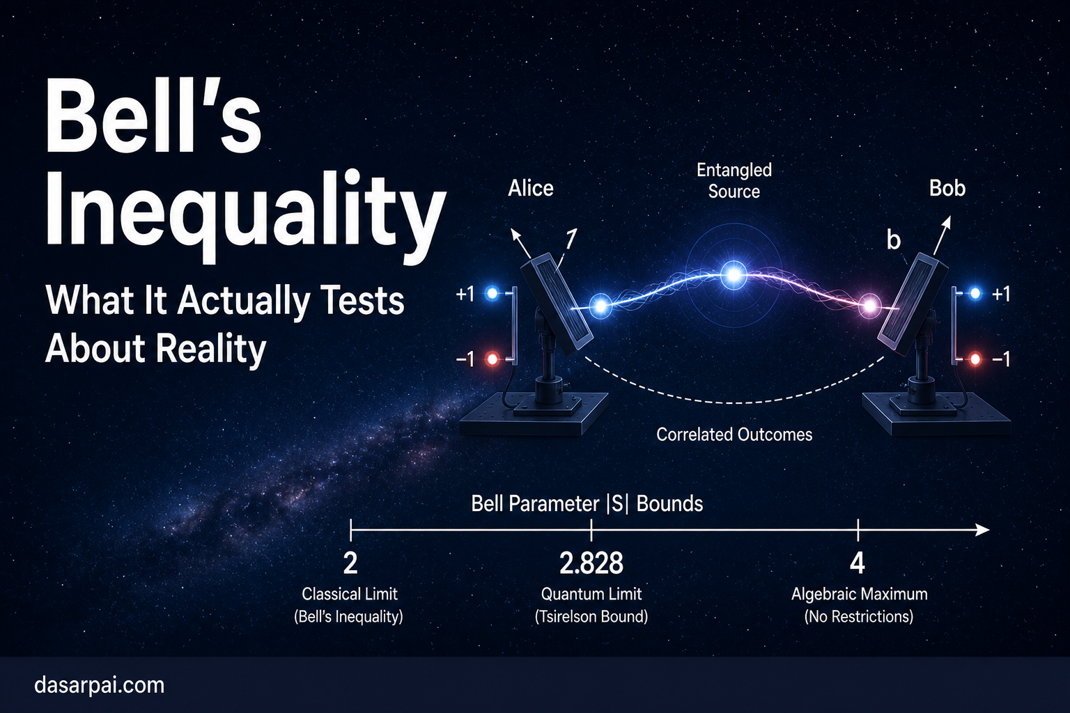
Imagine a source in the middle that repeatedly creates pairs of particles and sends them in opposite directions.
Alice  ←──── particle-pair source ───────→  Bob
         \                             /
          \____ same entangled pair __/
Each trial follows the same loop:
| Step | Who | What happens |
|---|---|---|
| 1 | Source | Creates one entangled pair and sends particles apart |
| 2 | Alice | Chooses a measurement direction, gets +1 or −1 |
| 3 | Bob | Chooses a measurement direction, gets +1 or −1 |
| 4 | Both | Write one row in the log — then discard the pair |
| 5 | Repeat | Thousands of fresh pairs; never re-measure the same pair |
That is the whole physical setup. Everything else is about what Alice and Bob choose to measure and what numbers they record.
2. What are Alice and Bob measuring?#
We will use electron spin as the example, but the logic applies to other quantum properties too.
Each particle flies toward Alice or Bob. That direction of travel is not the measurement direction.
The measurement direction is the orientation of the measuring device — the axis along which we ask a yes/no question:
“Is your spin aligned with this axis, or opposite to it?”
   Device A1 (vertical)          Device A2 (horizontal)

        ↑  axis                         ───→  axis
        │                                    │
        ●  electron                          ●  electron
Every measurement gives exactly one of two outcomes:
| Symbol | Meaning |
|---|---|
| +1 | spin-up along the chosen axis |
| −1 | spin-down along the chosen axis |
Key point: the measurement direction belongs to the apparatus, not to the direction the particle is traveling.
3. Two choices for Alice, two for Bob#
Alice can pick between two measurement directions: A1 and A2.
Bob can pick between B1 and B2.
Example (exact angles do not matter yet):
| Person | Setting | Example angle |
|---|---|---|
| Alice | A1 | 0° |
| Alice | A2 | 90° |
| Bob | B1 | 45° |
| Bob | B2 | −45° |
On any trial, Alice picks one setting and Bob picks one. That gives four possible combinations — and four correlations we will later combine:
| Combination | Alice uses | Bob uses | Correlation symbol |
|---|---|---|---|
| 1 | A1 | B1 | E(A1, B1) |
| 2 | A1 | B2 | E(A1, B2) |
| 3 | A2 | B1 | E(A2, B1) |
| 4 | A2 | B2 | E(A2, B2) |
These four terms are exactly why Bell’s inequality has four pieces.
Settings are not results#
This distinction matters throughout the rest of the article.
| Concept | Symbol example | What it is | Possible values |
|---|---|---|---|
| Setting | A1, B2 | Direction chosen by the device | one of two labels |
| Single-trial result | X₃(A1), Y₃(B2) | Outcome on trial 3 | +1 or −1 |
| Correlation | E(A1, B1) | Average pattern over many trials | −1 to +1 |
A1 does not mean “Alice got spin-up.” It only means “Alice measured along her first axis.”
For trial number n:
Xn(A1)  =  Alice's result on trial n when she used A1
Yn(B1)  =  Bob's result on trial n when he used B1
Each result is +1 or −1. E(A1, B1) is the statistical correlation built from many such trials.
4. What gets recorded?#
Think of the experiment as building a spreadsheet. Each row is one particle pair:
| Trial | Alice setting | Alice result | Bob setting | Bob result | Product (Alice × Bob) |
|---|---|---|---|---|---|
| 1 | A1 | +1 | B2 | −1 | −1 |
| 2 | A2 | −1 | B1 | −1 | +1 |
| 3 | A1 | +1 | B1 | +1 | +1 |
| 4 | A2 | +1 | B2 | −1 | −1 |
The Product column is how we detect correlation (see §5). We only include rows where the setting pair matches — trial 1 and 3 both use A1, but trial 1 paired A1 with B2 while trial 3 paired A1 with B1, so they belong to different correlation buckets.
In the background, the source should prepare the same kind of quantum state every time — for example, a particular entangled pair.
5. Correlation in plain language#
Focus on one setting pair — say Alice uses A1 and Bob uses B1. Filter the log to only those rows, then multiply outcomes:
| Alice result | Bob result | Product | Pattern |
|---|---|---|---|
| +1 | +1 | +1 | same |
| +1 | −1 | −1 | opposite |
| −1 | +1 | −1 | opposite |
| −1 | −1 | +1 | same |
Take the average of all products from trials with settings (A1, B1). That average is E(A1, B1).
Worked example — suppose five (A1, B1) trials gave:
| Trial | Alice | Bob | Product |
|---|---|---|---|
| 3 | +1 | +1 | +1 |
| 7 | +1 | −1 | −1 |
| 12 | −1 | −1 | +1 |
| 18 | +1 | +1 | +1 |
| 25 | −1 | +1 | −1 |
E(A1, B1) = (+1 − 1 + 1 + 1 − 1) / 5 = 0.2
E always lies between −1 and +1:
| E value | Meaning |
|---|---|
| +1 | outcomes always match |
| −1 | outcomes always opposite |
| 0 | no overall pattern |
Bell’s test is not about one measurement. It is about patterns across thousands of pairs.
Because Alice has two settings and Bob has two, we compute four correlations — one per row in the combination table in §3:
E(A1, B1) E(A1, B2) E(A2, B1) E(A2, B2)
6. The Bell score (CHSH form)#
Combine the four correlations into one number:
S = E(A1,B1) + E(A1,B2) + E(A2,B1) − E(A2,B2)
Then take the absolute value |S|.
Important: we do not take absolute values of the individual E terms first. We build S, then take |S|.
Worked example — algebra only#
Suppose the four correlations happen to be:
| Term | Value |
|---|---|
| E(A1, B1) | +1 |
| E(A1, B2) | +1 |
| E(A2, B1) | +1 |
| E(A2, B2) | −1 |
| Step | Calculation |
|---|---|
| Substitute | S = (+1) + (+1) + (+1) − (−1) |
| Add | S = 4 |
| Absolute value | |S| = 4 |
If the four E values were completely unrelated numbers between −1 and +1, pure algebra allows:
| Bound | Range |
|---|---|
| S | −4 to +4 |
| |S| | 0 to 4 |
So why does Bell claim |S| ≤ 2?
That is the heart of the theorem — and it comes from an assumption about how nature works, not from arbitrary math.
7. The classical picture: instruction sheets#
Before Bell, many physicists (Einstein among them) wondered whether quantum randomness was really just ignorance — like not knowing whether a coin under a cup is heads or tails before you lift the cup.
The coin already has a definite side. You just do not know it yet.
A local hidden-variable theory tries the same idea for quantum particles:
Each particle leaves the source carrying a hidden “instruction sheet” that fixes the answer for every measurement direction Alice or Bob might choose.
        SOURCE                         ALICE's particle
           │                    ┌──────────────────────────┐
           │                    │  If A1 asked → answer +1 │
           ├──── pair ────────→ │  If A2 asked → answer −1 │
           │                    └──────────────────────────┘
           │
           │                    ┌──────────────────────────┐
           └──── pair ────────→ │  If B1 asked → answer +1 │  → BOB
                                │  If B2 asked → answer +1 │
                                └──────────────────────────┘
One pair’s hidden sheet might look like this:
| Particle | If measured along… | Predetermined answer |
|---|---|---|
| Alice’s | A1 | +1 |
| Alice’s | A2 | −1 |
| Bob’s | B1 | +1 |
| Bob’s | B2 | +1 |
On any trial, Alice picks one setting and Bob picks one. The answers to the unchosen settings still exist — they were just never revealed.
Two assumptions sit behind this picture:
| Assumption | Plain-language meaning |
|---|---|
| Realism (narrow sense) | Outcomes are definite before anyone looks |
| Locality | Alice’s choice here cannot instantly rewrite Bob’s distant result |
Bell asked: if reality works this way, what correlations are mathematically possible?
8. Why instruction sheets cap |S| at 2#
For one hidden instruction sheet, write Alice’s predetermined answers as X(A1), X(A2) and Bob’s as Y(B1), Y(B2). Each is +1 or −1.
Define:
s = X(A1)·Y(B1) + X(A1)·Y(B2) + X(A2)·Y(B1) − X(A2)·Y(B2)
Group Bob’s terms:
s = X(A1)·[Y(B1) + Y(B2)] + X(A2)·[Y(B1) − Y(B2)]
Bob’s two answers can only be +1 or −1 — so only two cases exist:
| Case | Bob’s hidden answers | Y(B1) + Y(B2) | Y(B1) − Y(B2) | Which bracket is ±2? |
|---|---|---|---|---|
| A | Y(B1) = Y(B2) | ±2 | 0 | first (with X(A1)) |
| B | Y(B1) = −Y(B2) | 0 | ±2 | second (with X(A2)) |
In either case, one bracket is zero and the other is ±2. Since X(A1) and X(A2) are also ±1:
s = +2 or s = −2 → |s| = 2 for one instruction sheet
Averaging over many pairs with different hidden sheets spreads the value across [−2, +2], but never beyond:
|S| ≤ 2 ← Bell's inequality (CHSH form)
Why algebra allows 4 but instruction sheets cannot: four unrelated E values like (+1, +1, +1, −1) can give |S| = 4 on paper. But if all four E values must come from one consistent hidden sheet on each trial, they are tied together — that shared structure is what caps |S| at 2.
9. What quantum mechanics predicts#
Quantum mechanics describes particle pairs in entangled states. For a suitable entangled pair and suitable angle choices, it predicts:
|S| = 2√2 ≈ 2.828
That is above Bell’s classical cap of 2, but still below the algebra-only maximum of 4.
Three limits on a number line:
  0        2        2.828              4
  |--------|----------|----------------|
           ↑          ↑                  ↑
      classical    quantum           pure algebra
       cap |S|    cap |S|            cap |S|
| Source | Upper bound on |S| | What it assumes |
|---|---|---|
| Pure algebra | 4 | Four unrelated numbers |
| Local instruction sheets | 2 | Hidden answers + locality |
| Quantum mechanics (Tsirelson bound) | 2√2 ≈ 2.828 | Entangled quantum state |
Bell proved the classical line. Quantum theory supplied the second. Experiments had to choose.
10. What experiments found#
Starting in the 1970s — and with steadily tighter tests since — Bell experiments have measured these correlations with entangled photons, ions, and other systems.
| Stage | Who / when | Result |
|---|---|---|
| Theory | Bell (1964) | If local instruction sheets → |S| ≤ 2 |
| Prediction | Quantum mechanics | |S| can reach 2√2 |
| Early tests | Aspect et al. (1980s) | |S| > 2, consistent with QM |
| Modern tests | Many groups | Violations confirmed with high confidence |
The consistent experimental outcome:
|S| > 2 (values near 2.828 for optimal setups)
Conclusion: nature’s correlations cannot be fully explained by particles carrying complete local instruction sheets for every possible measurement.
11. What Bell rules out — and what it does not#
| Question | Answer |
|---|---|
| Are local hidden instruction sheets enough? | No — ruled out |
| Does Bell prove faster-than-light messaging? | No |
| Does Bell pick one interpretation of QM? | No |
| Does Bell show entangled particles correlate? | They correlate — but that alone is not the surprise |
What is ruled out#
Bell experiments rule out local hidden-variable theories — the combination of definite pre-existing answers and no instant influence from Alice’s distant choice on Bob’s outcome. At least one part of that classical picture must give way.
What is not ruled out#
| Claim | Verdict |
|---|---|
| Usable faster-than-light phone | Not supported |
| “Everything connected instantly” | Too vague; not what Bell tests |
| Consciousness collapses the wavefunction | Not addressed |
| Reality does not exist | Not addressed |
| One specific QM interpretation is correct | Not decided |
No faster-than-light phone: Alice cannot control whether she gets +1 or −1 on a given trial. Bob sees his own random-looking sequence. Only when they later compare notes through ordinary (light-speed-limited) communication do the correlations appear.
Different interpretations respond differently — some drop pre-existing definite values, some accept nonlocal influences, some question how “free” the setting choices are. Bell’s theorem narrows the menu; it does not pick the dish.
A note on “superposition”#
Physicists often say a particle is “in a superposition” before measurement. That describes the mathematical state used to calculate probabilities. Whether that state is reality itself, or information about reality, or something else is a separate question.
Bell’s result does tell us one thing clearly: quantum uncertainty is not ordinary ignorance of local, pre-existing properties. The hidden-coin story fails if the coin’s properties must also be local.
12. Why this theorem changed physics#
Before Bell, the Einstein–Bohr debate about quantum completeness could sound purely philosophical.
Bell turned it into checkable arithmetic:
“If Einstein-style local hidden explanations exist, then |S| ≤ 2. Go measure S.”
That is what makes the theorem remarkable. A question about the structure of reality became an experimental scoreboard.
The deepest surprise is not that distant particles correlate strongly — classical objects can correlate too. The surprise is the pattern across different measurement settings: a pattern no system of local pre-written answers can reproduce.
Nature does not fit inside the intuitive picture where
objects possess all relevant properties beforehand
        +
distant outcomes are independent of remote measurement choices
Quantum mechanics predicts the correlations with extraordinary accuracy. Bell tells us which classical explanation cannot work. What lies beneath that — information, reality, relations, branches, or something not yet named — is where the deepest questions still live.
Hashtags#
#BellsInequality #QuantumMechanics #QuantumEntanglement #LocalHiddenVariables #CHSHInequality #QuantumPhysics #PhilosophyOfScience #EinsteinBohrDebate #TsirelsonBound #PhysicsExplained #ScienceForEveryone #FoundationsOfQuantumMechanics

Comments: