
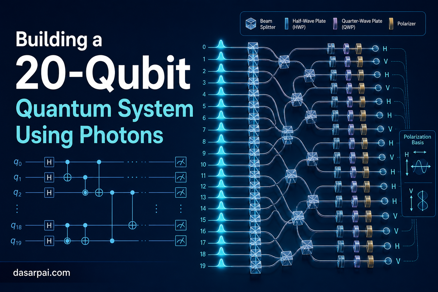
Building a 20-Qubit Quantum System Using Photons#
Part 13 of the Learning Quantum Physics series.
Quantum computing often becomes difficult to understand because we start directly with symbols such as:
|0>, |1>, superposition, entanglement, Hilbert space, and quantum gates.
A simpler approach is to start with the physical system — the actual hardware — and only then attach the math.
Let us assume that we want to build a 20-qubit quantum system using photons.
The central idea is:
One photon can be used as one qubit if we choose one two-state property of that photon to represent
|0>and|1>.
For this article, we will use the polarization of a photon.
If you write software#
If you already think in bits, registers, and logic gates, here is the mapping this article uses:
| Classical computing | Photonic qubits (this article) |
|---|---|
One bit: 0 or 1 | One qubit: two basis states labeled |0> and |1> |
| 20-bit register: one of 2^20 bit strings | 20-qubit register: one joint state in a 2^20-dimensional vector space |
| AND / OR / NOT gates | Unitary transforms implemented with wave plates, beam splitters, and phase shifters |
| Read register → get 20 bits | Measure 20 qubits → get one 20-bit outcome per experimental run |
The goal is not to memorize optics. It is to see where the symbols in a quantum circuit come from physically — so notation like |0>, |+>, tensor products, and entanglement map to hardware you could, in principle, build in a lab.
Throughout, |0> and |1> are Dirac ket labels (basis state names), not ASCII angle brackets around integers.
1. First, what exactly is the physical object?#
Our physical object is a photon.
A photon has several measurable properties, such as:
- polarization
- frequency
- direction of travel
- arrival time
- spatial mode
To create a qubit, we choose a physical property that can provide two distinguishable basis states.
For example, using polarization:
Horizontal polarization = |0>

Vertical polarization   = |1>
So the photon is the physical object.
Its polarization is the physical property we use.
And:
|0>
and
|1>
are mathematical labels representing two selected polarization states.
This distinction is important.
A photon is not literally a 0 or 1.
We are defining two physical states and assigning mathematical symbols to them.
2. One photon becomes one qubit#
Suppose we prepare one photon.
If it has horizontal polarization, we represent its state as:
|0>
If it has vertical polarization:
|1>
But quantum mechanics also allows the photon to be prepared in a superposition such as:
|+> = (|0> + |1>) / sqrt(2)
This does not mean that we have two photons.
We still have only one photon.
Its polarization state is represented by a combination of the two basis states.
Conceptually:
3. From one photon to twenty photons#
If one photon represents one qubit, then the simplest picture of a 20-qubit photonic system is:
Photon 1  → Qubit 1

Photon 2  → Qubit 2

Photon 3  → Qubit 3

...

Photon 20 → Qubit 20
We now have twenty physical quantum systems.
A simplified optical layout might look like this:
Photon 1   ─────────────────────

Photon 2   ─────────────────────

Photon 3   ─────────────────────

...

Photon 20  ─────────────────────
Each line may represent a separate optical path.
These are similar to the qubit wires we see in quantum circuit diagrams.
4. Step One: Generate twenty photons#
The first challenge is producing photons in a controlled way.
Ideally, we want:
Source 1 → exactly one photon

Source 2 → exactly one photon

...

Source 20 → exactly one photon
Real photonic systems may use technologies such as:
- quantum-dot single-photon sources
- spontaneous parametric down-conversion
- heralded photon sources
- other single-photon emitters
The engineering challenge is that we want a reliable quantum system.
For a particular optical mode, we do not want an unpredictable mixture of:
0 photons
or
1 photon
or
2 photons
when the computation requires exactly one.
Conceptually:
5. Step Two: Make the photons sufficiently indistinguishable#
Suppose we produce two photons.
One arrives slightly earlier than the other.
Or one has a slightly different frequency.
Or their pulse shapes differ.
Then they may become physically distinguishable.
This matters because quantum interference depends heavily on indistinguishability.
For photons to interfere properly, we may need to carefully control properties such as:
- frequency
- arrival time
- spatial mode
- spectral shape
- pulse duration
We still keep some selected property, such as polarization, available to encode the qubit.
So there is an important distinction.
We may want the photons to be indistinguishable in many physical properties while allowing their polarization states to carry quantum information.
For example:
Photon A:

same frequency
same arrival time
same spatial mode
polarization = H
and
Photon B:

same frequency
same arrival time
same spatial mode
polarization = V
Their polarization may differ while the other properties are tightly controlled.
6. Step Three: Define the computational basis#
Now we establish our convention:
Horizontal = |0>

Vertical   = |1>
Suppose all twenty photons are horizontally polarized.
The twenty-qubit state is:
|00000000000000000000>
This means:
Photon 1  → H
Photon 2  → H
Photon 3  → H
...
Photon 20 → H
Another possible state could be:
|10110001001010101101>
Each position corresponds to one photon’s polarization state.
For example:
1 → Vertical
0 → Horizontal
1 → Vertical
1 → Vertical
...
At this stage, however, we are still dealing with ordinary computational-basis states.
The more interesting quantum behavior begins when we create superpositions and interference.
7. Step Four: Put a photon into superposition#
A photon’s polarization can be changed using optical components.
A common device is a wave plate.
Using an appropriate wave plate, we can transform:
|0>
into:
(|0> + |1>) / sqrt(2)
which we call:
|+>
Conceptually:
This is somewhat analogous to applying a Hadamard gate in the circuit model.
For one qubit:
H|0> = |+>
where:
|+> = (|0> + |1>) / sqrt(2)
8. Put all twenty photons into superposition#
Now imagine applying the same operation to all twenty photons.
Each photon becomes:
|+>
The joint state is:
|+>|+>|+> ... |+>
twenty times.
We often write this compactly as:
|+>^⊗20
This notation simply means:
Take the tensor product of twenty
|+>states.
Software engineer’s view: If one qubit’s state lives in a 2-dimensional vector space, two independent qubits live in a 4-dimensional joint space (2 × 2). For twenty qubits, you take that tensor product twenty times — the same combinatorial idea as the Kronecker product of basis vectors in linear algebra:
dim(joint state) = 2 × 2 × ... × 2 (20 times) = 2^20
You are not storing 2^20 numbers in ordinary RAM after one measurement. Before measurement, the system is described by one complex amplitude vector that assigns a weight to each of the 2^20 possible basis labels.
Now something mathematically remarkable happens.
Each qubit has two basis states.
Therefore:
1 qubit  → 2 basis states

2 qubits → 4 basis states

3 qubits → 8 basis states

...

20 qubits → 2^20 basis states
And:
2^20 = 1,048,576
So a system consisting of only twenty qubits has a state space with:
1,048,576 computational basis states.
9. What does this large number really mean?#
It is easy to misunderstand this — especially if you think in terms of memory allocation.
It does not mean that we need:
1,048,576 photons
We still have only:
20 photons
Classical analogy: A 20-bit CPU register also holds one of 2^20 possible bit strings. The difference is not the count of labels — it is that a quantum register can exist in a superposition over those labels at once, with complex amplitudes that can interfere. A classical register always holds exactly one bit string.
But their joint quantum state is represented in a vector space having:
2^20
dimensions.
The state may therefore be written conceptually as:
c0 |00000000000000000000>

+ c1 |00000000000000000001>

+ c2 |00000000000000000010>

+ ...

+ c1048575 |11111111111111111111>
where every:
ci
is a complex amplitude.
This is the mathematical state description of the twenty-photon quantum system.
10. The important word is “joint”#
This is one of the most important ideas in quantum computing.
We should not think only about:
Photon 1 has its state.

Photon 2 has its state.

Photon 3 has its state.
After suitable quantum operations, the twenty photons may form one joint quantum state.
The system itself must then be described collectively.
This is where entanglement becomes possible.
11. Step Five: Make photons interfere#
Photons present a special engineering problem.
They are excellent at travelling without interacting strongly with the environment.
That is one reason they are attractive for quantum communication.
But this is also a difficulty.
Photons normally do not strongly interact with other photons.
Two photons can pass through each other without behaving like two strongly interacting particles — there is no easy “photon AND gate” wired like a transistor.
Quantum computation, however, needs operations that establish relationships between qubits.
So photonic quantum computing often uses interference rather than relying on direct photon-photon interactions.
One of the most important optical devices is the beam splitter.
Conceptually:
A beam splitter does more than simply split classical light.
For individual indistinguishable photons, quantum amplitudes associated with alternative paths can interfere.
This interference is one of the fundamental resources used in photonic quantum computing.
12. Why indistinguishability matters#
Suppose two photons arrive at a beam splitter.
If we can determine which photon followed which path, then some quantum alternatives become distinguishable.
That can destroy the interference we wanted.
But when the alternatives remain indistinguishable, their probability amplitudes can interfere.
So successful photonic quantum computation requires extremely precise control over:
Which alternatives can nature distinguish?
and:
Which alternatives remain coherent?
This is a deeper way of understanding why optical alignment, timing, frequency matching, and isolation are so important.
13. Step Six: Create entanglement#
Consider two photons.
A simple entangled state is:
(|00> + |11>) / sqrt(2)
This does not mean:
Photon A independently has 50% chance of 0 or 1

and

Photon B independently has 50% chance of 0 or 1.
The important feature is the relationship between them.
The two-photon system is described jointly.
When measured in the computational basis, the outcomes are correlated:
00
or:
11
with the corresponding probabilities.
But:
01
and:
10
do not appear for this ideal state.
14. A twenty-photon entangled state#
The same principle can be extended to more photons.
For example, consider:
(
|00000000000000000000>
+
|11111111111111111111>
)
/ sqrt(2)
This is an example of a twenty-qubit GHZ-type state.
It contains two coherent alternatives:
All twenty photons are in |0>
and:
All twenty photons are in |1>
The important thing is that these are not merely classical alternatives.
Their amplitudes form a coherent quantum superposition.
15. What would the physical machine contain?#
A conceptual photonic quantum computer might contain:
The real system might use many additional components.
But this diagram captures the basic idea.
16. Where are quantum gates physically?#
When we draw a quantum circuit, we might write:
|0> ── H ─────────

|0> ─────── CNOT ─

...
These symbols are mathematical abstractions — like pseudocode or a QASM instruction in a simulator.
In a photonic machine, the physical implementation may involve:
Hadamard-like operation
        ↓
wave plate
or
beam splitter
depending on encoding
and:
phase operation
        ↓
phase shifter
while two-qubit operations may require more elaborate interference networks, ancillary photons, and measurement.
So:
Quantum circuit gate
is the mathematical operation.
And:
optical hardware
is its physical implementation.
17. Measurement#
Eventually, we want information from the quantum system.
So the photons are sent to detectors.
For polarization encoding, the optical system can separate different polarizations before detection.
Conceptually:
For twenty photons, one experimental run may produce a classical result such as:
10110001001010101101
This is now ordinary classical information.
The quantum state has been measured in the chosen basis.
18. One run does not reveal the full quantum state#
This is another essential point.
Suppose the state contains amplitudes associated with more than one million basis states.
When we measure the twenty qubits, we do not receive all those amplitudes.
We obtain one outcome, for example:
00110100101011010001
We then repeat the experiment many times.
From the statistics of repeated measurements, together with the design of the algorithm, we learn useful information.
Quantum computation therefore does not mean:
Store one million classical answers and read them all at once.
That is not how quantum advantage works.
19. The photon does not have to use polarization#
So far we assumed:
Horizontal = |0>

Vertical = |1>
But this is only one possible physical encoding.
Photonic qubits can also use other degrees of freedom.
Path encoding#
Suppose the photon can travel through one of two paths:
Upper path = |0>

Lower path = |1>
Then a beam splitter can create:
photon in a coherent superposition of both paths
Conceptually:
Time-bin encoding#
Another possibility is arrival time.
For example:
early arrival = |0>

late arrival = |1>
The photon remains a single photon, but its temporal mode carries the qubit.
Frequency-bin encoding#
We might instead use two frequency modes:
frequency f0 = |0>

frequency f1 = |1>
Again, the qubit is encoded in a selected two-dimensional physical subspace.
20. Do we really need twenty separate photon sources?#
Not necessarily.
The simplest conceptual model is:
20 photons
+
20 optical paths
But modern photonic architectures can be more sophisticated.
For example, one source may emit photons at different times:
t1 → Photon 1

t2 → Photon 2

t3 → Photon 3

...

t20 → Photon 20
Different temporal modes can then play roles similar to separate circuit wires.
This is one reason the relationship between:
number of photons
and:
number of qubits
is not always as simple as it appears.
The exact answer depends on the encoding architecture.
21. A useful distinction: photon, mode, and qubit#
These three ideas should not be confused.
Photon#
A physical quantum of the electromagnetic field.
Mode#
A distinguishable optical degree of freedom, such as:
path
frequency
time
polarization
Qubit#
A selected two-dimensional quantum state space used for information processing.
Therefore:
physical object
        ↓
photon

available physical properties
        ↓
optical modes

selected two-state subspace
        ↓
qubit
22. Why twenty photons are difficult in practice#
The mathematics of adding qubits is easy:
20 qubits → 2^20 dimensions
But physically controlling twenty photons simultaneously is difficult.
One major reason is photon loss.
Suppose every photon’s probability of successfully surviving the complete experiment is:
90%
Then the probability that all twenty survive is:
0.9^20
which is approximately:
0.1216
or:
12.16%
So even though each photon individually has a very good survival probability, the probability of successfully retaining all twenty becomes much lower.
This is a powerful example of how small imperfections accumulate as quantum systems scale.
23. Other practical problems#
A real photonic quantum computer must deal with many engineering difficulties:
- imperfect photon sources
- photon loss
- detector inefficiency
- imperfect optical components
- phase instability
- timing errors
- frequency mismatch
- environmental noise
- unwanted distinguishability
- imperfect interference
The quantum circuit diagram hides all these physical details.
For example, a circuit may simply say:
Apply H
But the laboratory must actually make the corresponding optical transformation with extremely high precision.
24. The complete journey#
We can summarize the complete construction process as:
For our example:
Physical system:
20 photons

Encoding:
polarization

Basis:
H = |0>
V = |1>

Quantum state dimension:
2^20

Number of basis states:
1,048,576

Processing:
wave plates
beam splitters
phase shifters
interference

Output:
20 classical bits per measurement
25. From physical reality to mathematics and back#
We can now see the entire structure more clearly.
Notice that we continuously move between two levels.
Physical level#
There are:
photons
polarizers
wave plates
beam splitters
detectors
Mathematical level#
There are:
state vectors
complex amplitudes
tensor products
unitary transformations
probabilities
The mathematical model is extraordinarily powerful.
But the actual experiment is always performed by physical objects.
26. The most important insight#
The most remarkable fact is not simply that twenty photons can represent twenty bits.
A classical twenty-bit register can also represent one of:
2^20
possible bit strings.
The difference is that a quantum system can have a coherent joint state whose mathematical description contains amplitudes associated with those basis states.
For twenty qubits:
dimension = 2^20
For fifty qubits:
dimension = 2^50
For one hundred qubits:
dimension = 2^100
This exponential growth is one of the reasons quantum systems are so interesting computationally.
But the usefulness comes only when a quantum algorithm carefully controls:
superposition
+
phase
+
interference
+
entanglement
+
measurement
A quantum computer does not become powerful merely because a large state space exists.
The algorithm must manipulate that state space so that useful answers are enhanced and unwanted alternatives interfere destructively.
Final picture#
To build a 20-qubit system using photons, the conceptual process is:
Create photons
        ↓
Choose a two-state physical property
        ↓
Define |0> and |1>
        ↓
Prepare twenty qubits
        ↓
Create superposition
        ↓
Control phase
        ↓
Create interference
        ↓
Create entanglement when required
        ↓
Perform quantum operations
        ↓
Measure the photons
        ↓
Receive classical results
The twenty photons are the physical systems.
The qubits are the two-dimensional quantum information spaces encoded into those physical systems.
Together, the twenty qubits occupy a state space of dimension:
2^20 = 1,048,576
Yet physically we still have only a relatively small number of photons.
That gap between:
a small number of physical quantum systems
and:
an exponentially large joint state space
is one of the most beautiful ideas at the heart of quantum computing.
Hashtags#
#QuantumComputing #PhotonicQuantumComputing #Qubits #QuantumHardware #QuantumPhysics #LinearAlgebra #TensorProduct #QuantumEntanglement #SoftwareEngineering #PhysicsForEngineers #Optics #HilbertSpace

Comments: