
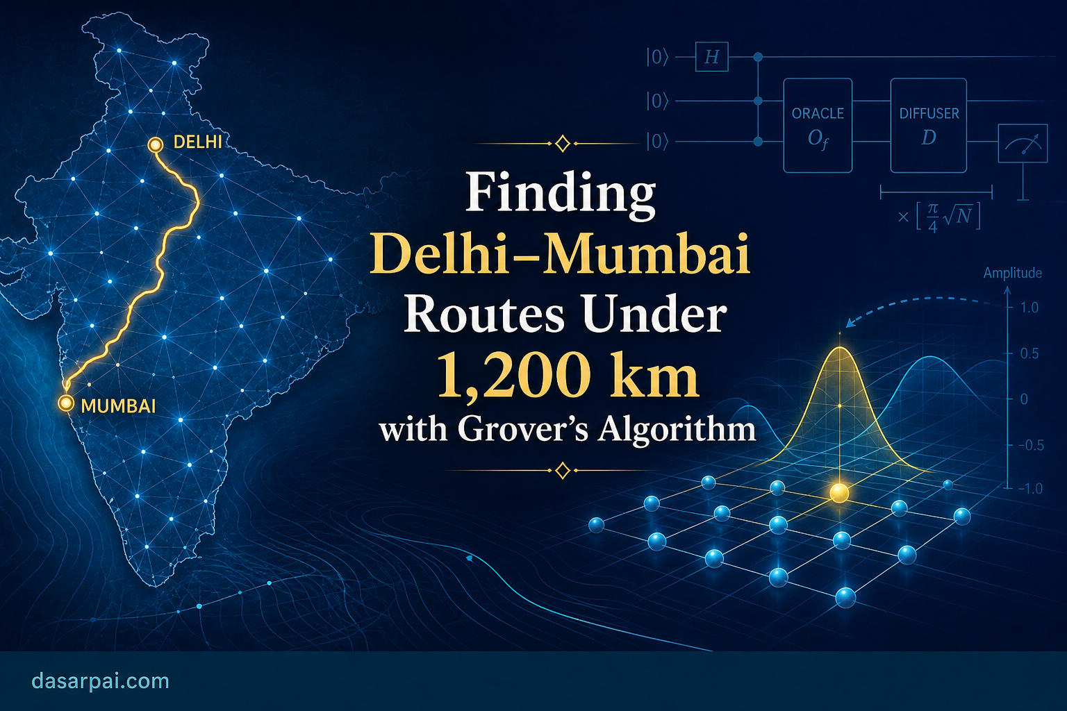
Finding Delhi–Mumbai Routes Under 1,200 km with Grover’s Algorithm#
Part 11 of the Learning Quantum Physics series.
Suppose we have 10,000 possible routes from Delhi to Mumbai. We want to find every route whose total length is less than 1,200 km.
It is tempting to say:
Put all 10,000 routes into superposition, apply Grover’s algorithm about \(\pi\sqrt{10{,}000}/4\) times, and measure the answer.
That sentence hides almost the entire problem.
Where did the 10,000 routes come from? How is a route represented? Where are the road distances stored? How does a quantum circuit add them? How does it test whether the sum is below 1,200? What if there are two or three qualifying routes? Does one measurement return all of them?
This article constructs the complete model without hiding those steps.
Who this article is for#
The intended reader is a software engineering professional: comfortable with graphs, arrays, binary numbers, Boolean predicates, and big-O reasoning, but not necessarily with quantum circuit design.
We use Delhi–Mumbai routing as a familiar domain example. This is not the traveling salesperson problem (TSP) in the usual sense—finding the single shortest tour through many cities. Here the classical world has already produced a fixed catalogue of 10,000 candidate routes. The quantum step is search: find which catalogue entries satisfy a predicate (total distance below 1,200 km). Think of it as accelerating repeated calls to a function such as is_under_1200_km(route_id) over an unstructured list, not as replacing Dijkstra or A* on a live road graph.
What we do not assume you already know: qubits, Dirac notation, Hadamard gates, phase oracles, reversible circuits, or amplitude amplification. Those ideas are introduced when they first matter.
1. What Grover’s algorithm actually solves#
Grover’s algorithm searches a finite set of candidates.
Let the candidates be numbered:
\[ x=0,1,2,\ldots,N-1. \]We also need a Boolean function:
\[ f(x)= \begin{cases} 1, & \text{if candidate }x\text{ satisfies the condition},\\ 0, & \text{otherwise.} \end{cases} \]For our route problem:
\[ f(x)=1 \]means:
Candidate route \(x\) is a legal Delhi–Mumbai route and its total distance is less than 1,200 km.
Grover’s algorithm does not automatically:
- discover the road network;
- create the candidate routes;
- obtain the distances;
- decide how routes are encoded;
- return every qualifying route in one measurement.
Those parts must be designed around Grover’s search procedure.
In classical code, the piece Grover accelerates is the predicate evaluation—the repeated yes/no test—not the upstream work of building the road graph or generating routes. The quantum oracle is the reversible circuit version of that predicate. It does not “know” the answer in advance; it marks candidate IDs that satisfy the condition so that later interference steps can amplify them.
The heart of Grover’s algorithm is not route planning. It is amplitude amplification once a suitable candidate set and oracle already exist.
2. First dataset: the road network#
We begin with a directed, weighted graph.
- A vertex represents a city or road junction.
- An edge represents a direct permitted connection.
- The weight of an edge is its distance in kilometres.
- If travel direction matters, \(A\to B\) and \(B\to A\) are separate edges.
For a small illustration, suppose the cities are:
| City ID | City |
|---|---|
| 0 | Delhi |
| 1 | A |
| 2 | B |
| 3 | C |
| 4 | D |
| 5 | Mumbai |
The road table might be:
| Edge ID | From | To | Distance | Connection? |
|---|---|---|---|---|
| 0 | Delhi | A | 60 km | 1 |
| 1 | Delhi | B | 90 km | 1 |
| 2 | A | B | 50 km | 1 |
| 3 | A | C | 100 km | 1 |
| 4 | B | C | — | 0 |
| 5 | B | D | 100 km | 1 |
| 6 | C | Mumbai | 900 km | 1 |
| 7 | C | D | 80 km | 1 |
| 8 | D | Mumbai | 850 km | 1 |
| 9 | A | Mumbai | 1,180 km | 1 |
The statement “B to C has no path” can be represented in either of two ways:
- omit \(B\to C\) from the edge table; or
- keep a complete city-pair table and store
connection = 0.
The first representation is normally more compact. The second can be easier when a circuit expects fixed-address records.
Adjacency and distance are different fields#
For each possible edge \(e\), define:
\[ a_e= \begin{cases} 1, & \text{if the direct road exists},\\ 0, & \text{otherwise,} \end{cases} \]and, when it exists, let:
\[ d_e=\text{distance of edge }e. \]We must not silently treat a missing road as a zero-kilometre road. Zero distance and no connection mean different things.
3. Second dataset: the candidate routes#
The road graph tells us which individual roads exist. It does not yet give us 10,000 complete Delhi–Mumbai routes.
A classical route-generation procedure must produce them. For example, it might use depth-first search, Yen’s algorithm, an application-specific rule, or an existing route catalogue. The generation rules must state whether:
- repeated cities are forbidden;
- repeated edges are forbidden;
- routes may contain toll roads;
- direction restrictions apply;
- a maximum number of stops is imposed;
- the 10,000 routes are all possible routes or only a selected set.
Without such restrictions, a graph containing a cycle may generate infinitely many walks. A vehicle could loop around the same cities repeatedly before reaching Mumbai. Therefore “there are 10,000 paths” is not a fact supplied by Grover; it is a property of the candidate-generation policy.
Example candidate-route table#
Using the small graph above:
| Route ID | Ordered cities | Edge IDs | Total distance |
|---|---|---|---|
| 0 | Delhi → A → C → Mumbai | 0, 3, 6 | 1,060 km |
| 1 | Delhi → A → C → D → Mumbai | 0, 3, 7, 8 | 1,090 km |
| 2 | Delhi → A → Mumbai | 0, 9 | 1,240 km |
| 3 | Delhi → B → D → Mumbai | 1, 5, 8 | 1,040 km |
Here the qualifying routes are IDs 0, 1, and 3.
They are below 1,200 km. Route 2 is not.
Two different binary representations#
Suppose we have ten possible edges. A route can be represented by a ten-bit edge-incidence vector.
For route 0, which uses edges 0, 3, and 6:
edge position: 9 8 7 6 5 4 3 2 1 0
route bits:    0 0 0 1 0 0 1 0 0 1
Thus a bit string such as 0001001001 means:
This particular route uses the edges whose positions contain 1.
It must not mean:
These are the roads that exist in the entire road network.
Road existence is shared graph data. Route membership is candidate-specific data.
There is another problem with an incidence vector: it records which edges are used but may lose their order. It can also represent disconnected edge collections that are not a route at all. Extra constraints are then needed to confirm that it forms one continuous Delhi–Mumbai path.
For a precomputed catalogue of 10,000 legal ordered routes, a simpler search key is therefore a route ID.
4. Direct notation, basis vectors, and state vectors#
4.1 Route numbers as ordinary integers#
Number the 10,000 routes:
\[ 0,1,2,\ldots,9999. \]This number is an index. It is not the distance and not the road pattern itself.
4.2 How many qubits are required?#
A qubit is the quantum analogue of a classical bit. Measured, it yields 0 or 1. Before measurement it can sit in a superposition—a weighted combination of both outcomes. One qubit has two basis labels, \(|0\rangle\) and \(|1\rangle\). Two qubits have four basis labels, \(|00\rangle, |01\rangle, |10\rangle, |11\rangle\), and so on.
Importantly, superposition is not the same as running four classical loops in parallel on separate hardware threads. All routes share one state vector; amplitudes interfere when we apply gates. Measurement still returns one route ID per run, with probabilities determined by those amplitudes.
With \(n\) qubits, the number of computational basis states is:
\[ 2^n. \]Now:
\[ 2^{13}=8192, \]which is too small, while:
\[ 2^{14}=16384. \]Therefore at least 14 qubits are needed for a binary route-ID register.
4.3 Direct, or Dirac, notation#
The notation is called Dirac notation.
The fourteen-qubit basis state
\[ |00000000000000\rangle \]represents route ID 0.
For example:
\[ 13=(00000000001101)_2, \]so route 13 is represented by:
\[ |13\rangle = |00000000001101\rangle. \]Route 9999 is:
\[ 9999=(10011100001111)_2, \]and is written:
\[ |9999\rangle = |10011100001111\rangle. \]The shorthand \(|x\rangle\) is usually clearer than repeatedly writing all fourteen bits.
4.4 Basis vector versus state vector#
A single basis state \(|x\rangle\) corresponds to a column vector of length \(2^{14}=16384\). It has one entry equal to 1 and every other entry equal to 0.
For example, schematically:
\[ |3\rangle= \begin{bmatrix} 0\\ 0\\ 0\\ 1\\ 0\\ \vdots \end{bmatrix}. \]The nonzero entry is at the position labelled 3, when counting from 0.
A general route-register state is:
\[ |\psi\rangle = \sum_{x=0}^{16383}\alpha_x|x\rangle. \]Here:
- \(\alpha_x\) is the complex amplitude of route ID \(x\) (a complex number, not a probability itself);
- \(|\alpha_x|^2\) is its measurement probability—the fraction of runs that would return ID \(x\);
- normalization requires
The state vector is therefore the column containing all 16,384 amplitudes.
It is not a classical array containing 16,384 readable routes. Measurement returns one basis-state label per run.
5. The important 10,000-versus-16,384 issue#
This point determines the iteration count.
A Hadamard gate (\(H\)) is the standard way to create an equal superposition from \(|0\rangle\). Applied to one qubit, \(H|0\rangle=(|0\rangle+|1\rangle)/\sqrt2\): both outcomes get equal amplitude. Applied independently to each qubit in a register, it creates a uniform superposition over all bit strings of that width—like initializing every index in a search array with equal weight before any predicate has been applied.
Fourteen Hadamard gates applied to \(|0\rangle^{\otimes14}\) create:
\[ |s_{16384}\rangle = \frac{1}{\sqrt{16384}} \sum_{x=0}^{16383}|x\rangle. \]But only IDs 0 through 9999 correspond to real route records. IDs 10000 through 16383 are padding states.
There are two honest designs.
Design A: exact superposition over 10,000 routes#
Prepare:
\[ |s_{10000}\rangle = \frac{1}{\sqrt{10000}} \sum_{x=0}^{9999}|x\rangle. \]Every valid route ID begins with amplitude:
\[ \frac{1}{\sqrt{10000}}=\frac{1}{100}. \]This makes \(N=10{,}000\), so the familiar estimate
\[ \frac{\pi}{4}\sqrt{10{,}000} = \frac{\pi}{4}\times100 \approx78.54 \]is relevant when exactly one route is marked.
However, exact uniform state preparation over a non-power-of-two number is not produced by fourteen plain Hadamard gates. A state-preparation circuit is required, and the diffusion operation must reflect about this prepared state.
Design B: use all 16,384 basis states#
Prepare the easy Hadamard superposition over all 16,384 IDs. The oracle rejects every padded ID.
Now the search space is:
\[ N=16{,}384, \]not 10,000. For one marked route, the estimate becomes:
\[ \frac{\pi}{4}\sqrt{16{,}384} = \frac{\pi}{4}\times128 \approx100.53. \]Therefore we cannot simultaneously say “use fourteen Hadamards over 16,384 states” and “the iteration count is based on 10,000” without further state-preparation logic.
For the main derivation below, we use Design A so that \(N=10{,}000\). The caveat about its preparation cost remains part of the complete algorithm.
6. Registers required by the quantum circuit#
The fourteen route qubits are not the whole computer. The oracle needs working registers.
One possible logical design is:
| Register | Purpose | Illustrative size |
|---|---|---|
| \(R\) | Route ID | 14 qubits |
| \(E\) | Current edge ID | depends on number of edges |
| \(A\) | Edge-available flag | 1 qubit |
| \(D\) | Current edge distance | enough bits for maximum edge distance |
| \(S\) | Running distance sum | enough bits for maximum possible route total |
| \(V\) | Valid-route flag | 1 qubit |
| \(C\) | Comparison result: sum < 1200 | 1 qubit |
| \(F\) | Final marked flag | 1 qubit |
| work | Carries, lookups, reversible arithmetic | circuit-dependent |
For example, eleven unsigned bits can store values from 0 through 2047. That is enough to store 1,200, but it is enough for the sum register only if the largest possible candidate-route total is no more than 2047 km.
If candidate routes might reach 10,000 km, fourteen sum qubits are needed because:
\[ 2^{13}=8192<10000, \]while:
\[ 2^{14}=16384>10000. \]Register sizes must follow declared data bounds. They cannot be chosen merely from the 1,200-km threshold.
7. What information the oracle must access#
For every route ID \(x\), the oracle needs enough data to determine:
- whether the record is a legal Delhi–Mumbai route;
- which ordered edges it contains;
- whether every selected edge exists;
- the distance of every edge;
- whether their sum is below 1,200 km.
There are two broad storage designs.
7.1 Store the already-computed total#
The classical candidate table contains:
route ID → ordered path, total distance, validity
The quantum oracle loads the total and compares it with 1,200.
This makes the oracle relatively small, but the distance summation has already been performed classically. Grover then accelerates only the search through the stored records.
7.2 Compute the total inside the oracle#
The route record contains its edge IDs. The oracle looks up each edge distance and reversibly adds it into the sum register.
This better exposes the computation, but it requires:
- coherent memory access or a compiled lookup circuit;
- reversible addition;
- route-length or termination encoding;
- validity checks;
- uncomputation of all temporary values.
Calling a conventional database through an ordinary classical API during a coherent superposition would measure or otherwise destroy the intended quantum computation. The data access must itself be implemented coherently—for example through a reversible lookup network or an assumed qRAM (quantum random-access memory) / qROM (quantum read-only memory) mechanism.
In software terms: you cannot call routes[route_id].distance from normal application code inside the quantum step and expect superposition to survive. The lookup table must be compiled into a reversible circuit that maps \(|route\_id\rangle|0\rangle \to |route\_id\rangle|distance\rangle\) without leaking which ID was queried into unrelated “garbage” qubits. Building that lookup at scale is often the dominant engineering cost.
That data-loading cost is a real part of the algorithm.
8. Building the reversible oracle step by step#
We now define the oracle for route ID \(x\).
The desired logical predicate is:
\[ f(x) = \operatorname{legal}(x) \land \bigl(L(x)<1200\bigr), \]where \(L(x)\) is the route’s total distance.
Step 1: start with clean work registers#
The input has the form:
\[ |x\rangle_R |0\rangle_E |0\rangle_D |0\rangle_S |0\rangle_V |0\rangle_C |0\rangle_F. \]Step 2: validate the route ID#
For exact 10,000-state preparation, every superposed ID is already between 0 and 9999. If padding is used, the circuit first checks:
\[ x<10000. \]It must also confirm that the stored record starts at Delhi, ends at Mumbai, contains a continuous ordered sequence, and satisfies the declared route rules—unless those properties were guaranteed when the candidate table was constructed.
Step 3: load one edge of the route#
For route position \(j\), perform a coherent lookup:
\[ |x\rangle|j\rangle|0\rangle_E \longrightarrow |x\rangle|j\rangle|e_{x,j}\rangle_E. \]Here \(e_{x,j}\) is the edge ID at position \(j\) in route \(x\).
Variable-length routes need a declared encoding, such as:
- a fixed maximum number of edges plus a route-length field; or
- a special end-of-route edge code.
Step 4: look up availability and distance#
Using the edge ID:
\[ |e\rangle|0\rangle_A|0\rangle_D \longrightarrow |e\rangle|a_e\rangle_A|d_e\rangle_D. \]If \(a_e=0\), the valid flag must become false. Again, a missing connection must not be treated as distance zero.
Step 5: add the edge distance#
Use a reversible adder:
\[ |S\rangle|d_e\rangle \longrightarrow |S+d_e\rangle|d_e\rangle. \]Repeat Steps 3–5 for every used edge.
For route 0 in the small example:
\[ S=0 \]becomes:
\[ 0+60=60, \]then:
\[ 60+100=160, \]and finally:
\[ 160+900=1060. \]Step 6: compare with 1,200#
A reversible comparator computes:
\[ C= \begin{cases} 1, & S<1200,\\ 0, & S\ge1200. \end{cases} \]The word less than matters. A route of exactly 1,200 km is rejected. If the intended condition is “not more than 1,200 km,” the comparator must instead test:
\[ S\le1200. \]Step 7: combine legality and comparison#
Compute:
\[ F=V\land C. \]Only a legal route below the threshold has \(F=1\).
Step 8: apply the phase mark#
The phase oracle performs:
\[ O_f|x\rangle = (-1)^{f(x)}|x\rangle. \]Therefore:
\[ f(x)=0 \quad\Rightarrow\quad |x\rangle\text{ is unchanged}, \]while:
\[ f(x)=1 \quad\Rightarrow\quad |x\rangle\mapsto-|x\rangle. \]The marked route does not yet have a higher probability. Only its phase—the sign of its amplitude—has changed.
That distinction matters for software intuition: after the oracle alone, measuring would still look nearly uniform. The probability boost comes only after diffusion combines these signed amplitudes through interference, much as signed values can cancel or reinforce before you take an absolute value.
Step 9: uncompute all work#
Run the arithmetic, lookups, and validity calculations backward so that every work register returns to zero:
\[ |x\rangle|\text{garbage}(x)\rangle \longrightarrow (-1)^{f(x)}|x\rangle|0\cdots0\rangle. \]This uncomputation is essential. Temporary registers must return to a clean \(|0\cdots0\rangle\) state so they do not remember route-specific details.
Software analogy: imagine a pure function mark_if_qualifying(route_id) that may use local variables and scratch buffers while it runs, but must leave no route-specific residue in global state when it returns. If distance sums or edge IDs remain written into work qubits, those qubits become entangled with the route register—linked so that measuring one reveals information about the other—and the standard diffusion step no longer acts on a uniform superposition over route IDs alone.
9. Preparing all 10,000 candidates#
Begin with the route register in:
\[ |0\rangle_R. \]Apply a state-preparation unitary \(A\)—a reversible quantum operation analogous to an invertible matrix multiply on the amplitude vector—such that:
\[ A|0\rangle = |s\rangle = \frac{1}{100} \sum_{x=0}^{9999}|x\rangle. \]Every route initially has amplitude:
\[ \alpha_x=\frac{1}{100}, \]and probability:
\[ P(x)=\left|\frac{1}{100}\right|^2 = \frac{1}{10000}. \]At this stage, measuring produces a uniformly random route. There is no preference for a route below 1,200 km.
The purpose of Grover iterations is to rotate amplitude toward the qualifying subspace.
10. The diffusion operation#
For a Hadamard-prepared power-of-two search space, diffusion is often written:
\[ D=2|s\rangle\langle s|-I. \]Conceptually it reflects every amplitude about the mean amplitude.
If \(A\) prepares the exact 10,000-state superposition, the corresponding reflection can be implemented as:
\[ D = A\bigl(2|0\rangle\langle0|-I\bigr)A^\dagger. \]This is another reason the exact state-preparation circuit matters. The diffuser must reflect about the state that was actually prepared.
One Grover iteration is:
\[ G=DO_f. \]In words:
- the oracle changes the sign of qualifying amplitudes;
- diffusion reflects all amplitudes about their mean;
- as a result, qualifying amplitudes grow and nonqualifying amplitudes shrink.
The process is interference, not parallel classical reading of all route records.
11. Why the search becomes a two-dimensional rotation#
Suppose exactly \(M\) of the \(N=10{,}000\) routes qualify.
Define the normalized state of all qualifying routes:
\[ |W\rangle = \frac{1}{\sqrt M} \sum_{x:f(x)=1}|x\rangle. \]Define the normalized state of all nonqualifying routes:
\[ |B\rangle = \frac{1}{\sqrt{N-M}} \sum_{x:f(x)=0}|x\rangle. \]The initial uniform state can be written:
\[ |s\rangle = \sin\theta\,|W\rangle + \cos\theta\,|B\rangle, \]where:
\[ \sin\theta = \sqrt{\frac{M}{N}}. \]Therefore:
\[ \theta = \arcsin\sqrt{\frac{M}{N}}. \]After \(r\) Grover iterations:
\[ G^r|s\rangle = \sin((2r+1)\theta)|W\rangle + \cos((2r+1)\theta)|B\rangle. \]Hence the probability of measuring some qualifying route is:
\[ P_{\text{success}}(r) = \sin^2((2r+1)\theta). \]This formula explains both the speed and the stopping point.
If we keep iterating after the probability has approached its maximum, the state rotates past the target and the success probability falls again. Grover amplification is oscillatory.
12. Where \(\pi\times100/4\) comes from#
We want:
\[ (2r+1)\theta \approx \frac{\pi}{2}. \]Solving for \(r\):
\[ r \approx \frac{\pi}{4\theta}-\frac12. \]When \(M\ll N\):
\[ \theta \approx \sqrt{\frac{M}{N}}. \]Therefore:
\[ r \approx \frac{\pi}{4} \sqrt{\frac{N}{M}}. \]If exactly one route qualifies#
Set:
\[ N=10000, \qquad M=1. \]Then:
\[ r \approx \frac{\pi}{4} \sqrt{10000} = \frac{\pi}{4}\times100 \approx78.54. \]The more accurate integer choice is about 78 Grover iterations.
Thus “\(\pi\times100/4\) iterations” is not a universal fact about the 10,000-route problem. It assumes:
- the effective search space contains exactly 10,000 equally weighted states;
- exactly one state is marked;
- the standard Grover rotation model applies.
If two routes qualify#
Now:
\[ M=2. \]The estimate is:
\[ r \approx \frac{\pi}{4} \sqrt{\frac{10000}{2}} \approx55.54. \]An appropriate integer is about 55 iterations.
If three routes qualify#
Now:
\[ M=3. \]Then:
\[ r \approx \frac{\pi}{4} \sqrt{\frac{10000}{3}} \approx45.34. \]An appropriate integer is about 45 iterations.
| Number of qualifying routes \(M\) | Approximate iterations |
|---|---|
| 1 | 78 |
| 2 | 55 |
| 3 | 45 |
More solutions require fewer iterations to amplify the qualifying subspace.
13. But we do not initially know whether M is 1, 2, or 3#
This is not a minor detail. The stopping time depends on \(M\), the number of answers, but finding \(M\) may itself be part of the problem.
Possible approaches include:
Approach 1: quantum counting#
Quantum counting estimates \(M\) by applying phase estimation—a separate quantum subroutine that reads properties of the Grover operator’s rotation angle—rather than by guessing iteration counts blindly. The estimate can then determine a suitable iteration count.
This requires extra circuitry and is not the same as ordinary Grover search.
Approach 2: unknown-solution search#
Algorithms for an unknown number of marked items choose varying or randomized Grover iteration counts. They can retain the quadratic-order advantage without first knowing the exact \(M\).
Approach 3: make a promise#
For a teaching example, we may explicitly promise:
Exactly one route in the candidate table is shorter than 1,200 km.
Only under that promise can we directly choose approximately 78 iterations.
Running 78 iterations when there are actually two or three answers can overshoot the ideal rotation and reduce the success probability. Therefore an article must not claim that the same 78 iterations automatically handles one, two, or three qualifying routes.
14. What measurement finally gives us#
After the chosen number of Grover iterations, measure the fourteen route-ID qubits.
Suppose the result is:
00000000001101
Convert it to decimal:
\[ (00000000001101)_2=13. \]The quantum computer has returned route ID 13.
It has not returned a human-readable route description. The classical route table is used to decode it:
route ID 13
→ Delhi → city A → city D → ... → Mumbai
→ stored or recomputed distance: 1,147 km
The result should then be verified classically:
- fetch route record 13;
- confirm that its first city is Delhi;
- confirm that its last city is Mumbai;
- confirm every consecutive road exists;
- recompute the sum of its edge distances;
- confirm that the sum is below 1,200 km.
Classical verification is inexpensive for one returned route and protects against implementation errors and hardware noise.
15. How do we obtain all two or three qualifying routes?#
One execution and one measurement produce one route ID.
If there are three qualifying routes, the amplified state is approximately:
\[ |W\rangle = \frac{1}{\sqrt3} \left( |x_1\rangle +|x_2\rangle +|x_3\rangle \right). \]Measurement returns one of them, approximately uniformly when the setup treats them symmetrically.
It does not print all three at once.
There are two main recovery strategies.
Strategy A: repeat and collect distinct answers#
Run the search again, measure again, verify the result, and store every new route ID in a classical set.
With three equally likely qualifying routes, repeated runs might return:
run 1 → route 27
run 2 → route 27
run 3 → route 814
run 4 → route 5302
After run 4, all three have been observed.
If \(M\) is known and marked answers are equally likely, the expected number of successful samples required to observe all \(M\) is approximately:
\[ M H_M, \]where \(H_M\) is the \(M\)-th harmonic number:
\[ H_M = 1 + \frac12 + \frac13 + \cdots + \frac1M. \]For example, \(H_3 = 1 + \frac12 + \frac13 \approx 1.83\), so if three qualifying routes are equally likely on each successful run, we expect roughly \(3 \times 1.83 \approx 5.5\) successful samples—not three—before we have seen every answer at least once, because the same route can appear twice before a missing one shows up. Repetitions can occur, so there is no fixed guarantee that exactly \(M\) runs will reveal all \(M\) answers.
Strategy B: exclude already-found routes#
After finding route \(x_1\), modify the oracle so that it marks:
\[ f(x)=1 \quad\text{and}\quad x\ne x_1. \]Run the search again to obtain another route. Continue excluding previously found IDs.
The number of remaining marked routes changes after each discovery, so the optimal Grover iteration count also changes.
To know that the list is complete, we need either:
- prior knowledge of \(M\);
- a counting procedure;
- or a declared probabilistic stopping rule.
Grover search alone does not announce, “there are no more answers.”
16. A complete small example before returning to 10,000 routes#
Use the four-route table from Section 3:
| ID | Total | Below 1,200? |
|---|---|---|
| 0 | 1,060 | 1 |
| 1 | 1,090 | 1 |
| 2 | 1,240 | 0 |
| 3 | 1,040 | 1 |
The route register needs two qubits because:
\[ 2^2=4. \]The initial uniform state is:
\[ |s\rangle = \frac12 \left( |00\rangle+|01\rangle+|10\rangle+|11\rangle \right). \]The oracle predicate is:
\[ f(0)=1, \quad f(1)=1, \quad f(2)=0, \quad f(3)=1. \]After phase marking:
\[ O_f|s\rangle = \frac12 \left( -|00\rangle -|01\rangle +|10\rangle -|11\rangle \right). \]This particular toy example has \(M=3\) answers out of \(N=4\). Standard Grover amplification is most visually intuitive when marked items are a small fraction of the search space; with three quarters already valid, random sampling is already very successful and ordinary iteration choices require care.
That observation is useful: Grover is most attractive when qualifying routes are rare.
For the 10,000-route case with only one, two, or three qualifying routes, the marked fraction is very small:
\[ \frac{1}{10000}, \qquad \frac{2}{10000}, \qquad \frac{3}{10000}. \]That is the regime in which the familiar square-root query reduction is meaningful.
17. The complete 10,000-route workflow#
We can now state every stage explicitly.
Classical preparation#
- Assign a unique ID to every city and road edge.
- Store every directed road connection and its distance.
- Declare what counts as a legal route.
- Generate or obtain exactly 10,000 candidate Delhi–Mumbai routes.
- Give each route an ID from 0 through 9999.
- Store each route as an ordered edge sequence.
- Choose whether totals are stored or computed inside the oracle.
- Define the exact predicate \(L(x)<1200\).
Quantum circuit construction#
- Allocate a fourteen-qubit route-ID register.
- Allocate distance, validity, comparator, and work registers.
- Build coherent route and edge lookup operations.
- Build reversible validation and addition circuits.
- Build the reversible less-than-1,200 comparator.
- Convert the Boolean result into a phase flip.
- Uncompute every temporary register.
- Build exact uniform state preparation over 10,000 IDs—or explicitly use a padded 16,384-state model.
- Build diffusion about the actually prepared initial state.
Search and recovery#
- Determine or estimate the number \(M\) of qualifying routes, or use an unknown-\(M\) search method.
- Apply the appropriate number of Grover iterations.
- Measure the route-ID register.
- Decode the binary result into a route ID.
- Retrieve and classically verify the route.
- Repeat if all qualifying routes, rather than one, are required.
18. Classical versus quantum query counts#
If exactly one qualifying route is hidden in an unstructured list of 10,000 records:
- a classical search may need up to 10,000 predicate evaluations—equivalent to calling
is_qualifying(route_id)up to 10,000 times in a linear scan; - it needs about 5,000 evaluations on average if the marked location is uniformly random and the search stops when it is found;
- Grover search needs on the order of \(\sqrt{10{,}000}=100\) oracle uses, with the more specific one-solution estimate near 78 iterations.
This \(\sqrt{N}\) versus \(N\) comparison is query complexity: it counts how many times the oracle predicate must be evaluated, not how many physical logic gates the full machine executes.
But one Grover iteration is not one elementary hardware gate.
It includes:
- route-data lookup;
- multiple edge lookups;
- reversible additions;
- comparisons;
- phase marking;
- uncomputation;
- diffusion.
Therefore the meaningful resource estimate is closer to:
\[ \text{iterations} \times \text{cost of one reversible oracle and diffuser}. \]The square-root advantage is a query-complexity result. It does not guarantee that a practical quantum machine will beat a classical shortest-path algorithm for this road problem.
19. Why Grover is not normally the first algorithm for road navigation#
Real road routing has structure. Distances live on a graph, and algorithms such as Dijkstra’s algorithm or A* exploit that structure. If edge weights are nonnegative and the goal is the shortest route, scanning an unstructured catalogue of 10,000 already-generated paths may be the wrong formulation.
Grover is appropriate for the teaching model when:
- the 10,000 candidates are already defined;
- they are treated as an unstructured set;
- testing a candidate is the main operation;
- qualifying candidates are rare;
- coherent access and a reversible oracle are available.
The honest conclusion is not “Grover is the best navigation algorithm.” It is:
Given a prepared set of 10,000 candidate routes and a reversible predicate that recognizes routes below 1,200 km, Grover’s method can amplify the qualifying route IDs using on the order of \(\sqrt{N/M}\) oracle calls.
That is precise, useful, and does not hide the engineering work.
20. Final answer to the original question#
If there are exactly 10,000 equally weighted candidate routes and exactly one is shorter than 1,200 km, the complete logical process is:
- represent the road system as a weighted directed graph;
- create a catalogue of 10,000 legal ordered Delhi–Mumbai routes;
- assign route IDs 0 through 9999;
- represent each ID with a fourteen-qubit computational basis state;
- prepare an exact uniform superposition over those 10,000 IDs;
- reversibly load or calculate each route’s distance in superposition;
- phase-flip only the IDs whose valid route total is below 1,200 km;
- uncompute the working data;
- apply diffusion;
- repeat the oracle-plus-diffusion operation about 78 times;
- measure one route ID;
- decode and verify that route classically.
If there are two qualifying routes, use about 55 iterations when \(M=2\) is known.
If there are three, use about 45 when \(M=3\) is known.
To recover all of them, repeat the complete search and measurement process, recording or excluding routes already found. One quantum measurement returns one route ID, not an entire list.
Finally, if fourteen ordinary Hadamard gates create a superposition over 16,384 basis states, then the effective \(N\) is 16,384 and the one-answer iteration estimate is about 100—not \(\pi\times100/4\). The latter belongs specifically to an effective 10,000-state search with one marked answer.
That distinction is the difference between a slogan about Grover’s algorithm and a complete algorithmic model.
Key notation at a glance#
| Symbol | Meaning |
|---|---|
| \(x\) | Candidate route ID |
| \(N\) | Number of states in the effective search space |
| \(M\) | Number of qualifying routes |
| ( | x\rangle) |
| ( | s\rangle) |
| \(L(x)\) | Total distance of route \(x\) |
| \(f(x)\) | 1 exactly when route \(x\) is legal and below 1,200 km |
| \(O_f\) | Phase oracle implementing \((-1)^{f(x)}\) |
| \(D\) | Diffusion/reflection operation |
| \(G=DO_f\) | One Grover iteration |
| \(r\) | Number of Grover iterations |
| \(\theta\) | Grover rotation angle, with \(\sin\theta=\sqrt{M/N}\) |
Further reading#
- Lov K. Grover, “A Fast Quantum Mechanical Algorithm for Database Search,” Proceedings of STOC, 1996.
- Michel Boyer, Gilles Brassard, Peter Høyer, and Alain Tapp, “Tight Bounds on Quantum Searching,” Fortschritte der Physik, 1998.
- Gilles Brassard, Peter Høyer, Michele Mosca, and Alain Tapp, “Quantum Amplitude Amplification and Estimation,” 2002.
Hashtags#
#GroversAlgorithm #QuantumComputing #QuantumSearch #SoftwareEngineering #RoutePlanning #GraphAlgorithms #Qubits #QuantumOracle #AmplitudeAmplification #QueryComplexity #QuantumAlgorithms #DelhiMumbaiRoutes

Comments: