
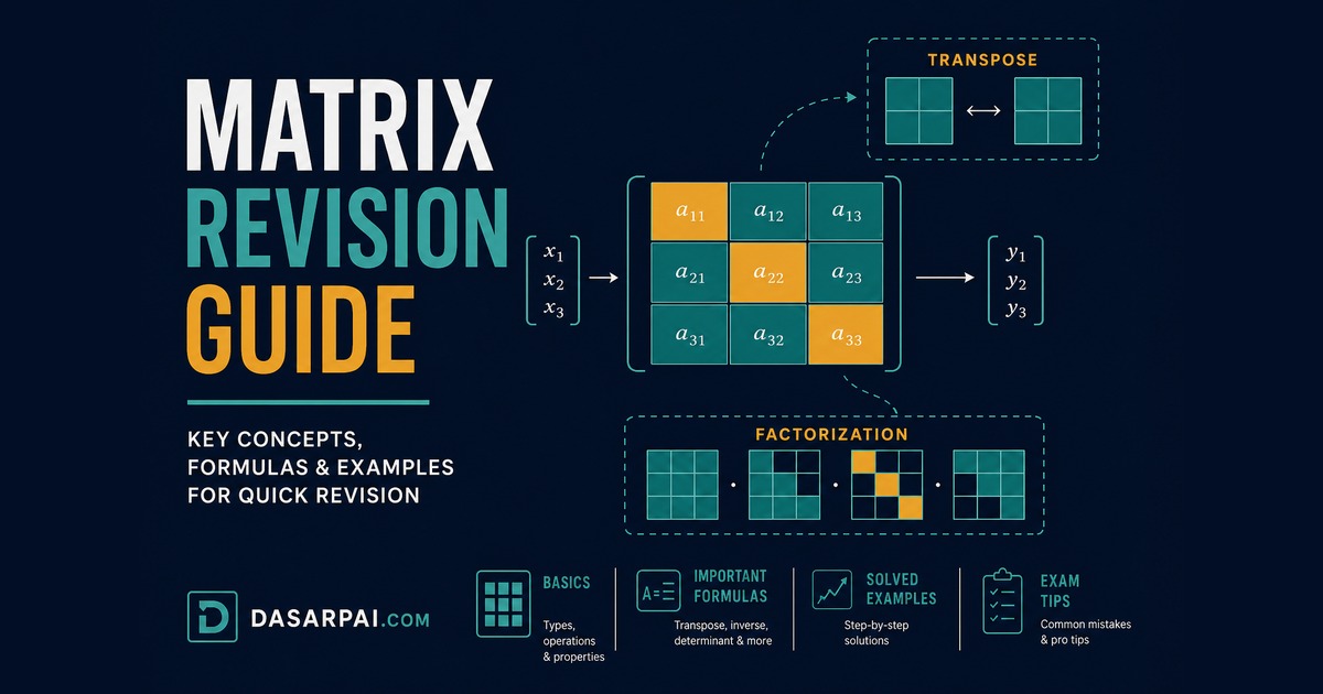
Matrices: A Complete Revision Guide#
Part 10 of the Learning Quantum Physics series.
This is a revision map for matrices, not a first-learning course. If you already know the definitions and just need to refresh the row-by-column rule, a determinant shortcut, or when to reach for an SVD instead of an eigendecomposition, skim the section you need and move on. For a final rapid refresh, skim the lookup tables at the end.
Each section below is deliberately short: a one-line definition, a tiny \(2\times2\) example where one helps, and a pointer to a deeper article when a topic deserves a full derivation. Sections 1–5 cover the building blocks — what a matrix is, the types worth recognizing by name, and the four basic operations. Later sections move through determinants, inverses, rank, eigenvalues, decompositions, and conditioning, ending with dense lookup tables for the day before an exam or an interview. Use the table of contents to jump straight to what you forgot, and use the MathJax formulas to check the exact form as you go.
1. Matrix foundations#
A matrix is a rectangular array of numbers with \(m\) rows and \(n\) columns, written \(m\times n\) — rows first, columns second, always in that order.
Each entry \(a_{ij}\) sits at row \(i\), column \(j\); the row index always comes before the column index.
Scalar — a single number, often represented by or closely related to a \(1\times1\) matrix. Vector — an \(n\times1\) (column) or \(1\times n\) (row) matrix. Matrix — the general rectangular case; a vector and a scalar are both special matrices.
Motivation — one array, many jobs. The same rectangular grid is not one thing. Depending on the job, a matrix may represent:
- a linear transformation — a map that sends every input vector to an output vector (§11);
- an operator — the same map, named that way in physics and functional analysis, acting on a state;
- a system of linear equations \(Ax=b\) (§9);
- a rotation — turning space without stretching it (§13);
- a scaling — stretching or shrinking along chosen directions (§11, §12);
- an observable in quantum mechanics — typically a Hermitian operator whose eigenvalues are the possible measurement outcomes;
- or some other linear relationship — covariance, adjacency, attention weights, a change of basis (§18).
That is why this guide exists: one object, many linear stories. Learn to read which story a given matrix is telling, and the formulas below become tools instead of a catalog. Two everyday readings still cover most of the work: a matrix as data (rows = records, columns = features, as in a spreadsheet or a design matrix) and a matrix as a linear map. Pick whichever makes a given formula easier to picture.
Here \(A\) is \(2\times2\); the entry \(a_{21}\) lives in row 2, column 1, and equals 3 — not to be confused with \(a_{12}=2\), the mirror entry across the diagonal.
Notation habit worth keeping: uppercase letters (\(A, B, X\)) for matrices, lowercase bold or arrowed letters for vectors, and plain lowercase for scalars and individual entries. It is a convention, not a rule, but sticking to it makes formulas easier to skim later.
2. Important matrix types#
Recognize these by name; only a handful get full treatment later.
- Shape: row (\(1\times n\)), column (\(n\times1\)), square (\(n\times n\)), rectangular (\(m\neq n\)).
- Special: zero matrix \(0\) (every entry zero); identity \(I\) (ones on the diagonal, zeros elsewhere — multiplying by \(I\) changes nothing, just like multiplying a number by 1); scalar matrix \(kI\) (a plain number \(k\) times the identity); diagonal (nonzero only on the diagonal).
- Triangular / band: upper triangular (zeros below the diagonal); lower triangular (zeros above); tridiagonal and other band matrices keep nonzero entries only near the diagonal — mentioned here, not expanded.
- Symmetry: a matrix is symmetric if flipping it across its main diagonal leaves it looking exactly the same, \(A^\top=A\) — like a butterfly’s two wings mirroring each other. It is skew-symmetric if that same flip flips every sign instead, \(A^\top=-A\); this forces every diagonal entry to be zero.
- Complex: Hermitian (\(A^*=A\), the complex analog of symmetric); unitary (\(U^*U=I\), the complex analog of orthogonal).
- Algebraic:
- Orthogonal \(Q^\top Q=I\): a rotation or a mirror-flip — it turns or flips things around but never stretches or squashes them, so lengths and angles stay exactly the same (full treatment in §13).
- Idempotent \(A^2=A\): like rounding a number that is already rounded — do it a second time and nothing changes further. Every projection, below, behaves this way.
- Involutory \(A^2=I\): like flipping a light switch twice — you land right back where you started, so it undoes itself. A mirror reflection behaves the same way.
- Nilpotent: fades to nothing if you repeat it enough times, even though it isn’t zero itself — like a photocopy of a photocopy of a photocopy, eventually turning blank. Example: \(\begin{bmatrix}0&1\\0&0\end{bmatrix}\) squares to the zero matrix.
- Projection: casts a shadow — it flattens something onto a smaller, flatter space and throws away the rest. Example: dropping the \(z\)-coordinate of a 3D point flattens it onto the \(xy\)-plane; doing that a second time gives the same flat result as doing it once.
- Permutation: a reshuffle — the same rows or columns, just rearranged, nothing added or removed. Example: swapping rows 1 and 2 of the identity matrix.
- Rank / determinant: a square matrix is nonsingular (equivalently invertible, or full rank) when \(\det(A)\neq0\), and singular when \(\det(A)=0\) — a singular matrix squashes at least one direction down to zero, which is exactly why it has no inverse. For example, \(\begin{bmatrix}1&2\\2&4\end{bmatrix}\) is singular (\(\det=1\cdot4-2\cdot2=0\); column 2 is just twice column 1, so no new direction is added), while \(\begin{bmatrix}1&2\\3&4\end{bmatrix}\) is nonsingular (\(\det=-2\neq0\)).
- Definiteness:
- Setup: \(A\) is a real, symmetric \(n\times n\) matrix — the same kind of matrix-as-a-map \(A\) from §11, just restricted to being symmetric. \(x\) is any nonzero vector of the matching size \(n\). Plugging \(x\) into both sides of \(A\), the product \(x^\top Ax\) always collapses to one plain number, since the shapes \((1\times n)(n\times n)(n\times1)\) multiply down to a single \(1\times1\) result.
- The picture: let \(x\) sweep through every possible direction and plot the resulting number \(x^\top Ax\) above each one — the result traces out a bowl-shaped surface.
- Positive definite: the bowl curves upward in every direction — \(x^\top Ax>0\) for every nonzero \(x\) — so there is one clear bottom and never a flat spot or a saddle.
- Positive semidefinite: a relaxed version of the same idea — the bowl is allowed to flatten out and touch zero (\(x^\top Ax\ge0\)) along some directions, instead of curving strictly upward everywhere.
- Example: with \(A=\begin{bmatrix}4&0\\0&9\end{bmatrix}\) and \(x=(x_1,x_2)\), \(x^\top Ax=4x_1^2+9x_2^2\), which is positive for every nonzero \(x\) — so this \(A\) is positive definite.
- Complex case: for a Hermitian matrix, the same bowl picture holds with \(x^*Ax\) in place of \(x^\top Ax\).
- Named structures (recognize only):
- Toeplitz: every diagonal running from top-left to bottom-right holds the same value, so the whole matrix is fixed by just its first row and first column.
- Vandermonde: each row is built from the powers of one number in a sequence, e.g. \(1,\,x_i,\,x_i^2,\,x_i^3,\ldots\) — the standard setup behind polynomial fitting and interpolation.
- Circulant: each row is the row above it, shifted over by one position and wrapped around — a Toeplitz matrix (above) with wraparound instead of running off the edge.
- Sparse: overwhelmingly zero entries — worth storing and computing with only the nonzero ones instead of the full grid.
- Jacobian: collects every first-order partial derivative of a vector-valued function \(f\) — one or more outputs, any number of inputs — into one matrix: row \(i\) holds the partial derivatives of output \(i\) with respect to every input. Example: for \(f(x,y)=(x^2+y,\ xy)\), which has 2 outputs and 2 inputs, the Jacobian is \(\begin{bmatrix}2x&1\\y&x\end{bmatrix}\), a \(2\times2\) matrix because there are 2 outputs and 2 inputs.
- Hessian: collects every second-order partial derivative of a scalar-valued function \(g\) — exactly one output — into one matrix; its definiteness (the “bowl” picture from just above) reveals whether a point is a minimum, a maximum, or a saddle of \(g\). The restriction to one output is essential: a function with 2 outputs would need one whole Hessian matrix per output (a stack of matrices, not a single one), so “the Hessian” only stays a single, clean matrix when there is one output to begin with. Put another way, the Hessian of \(g\) is just the Jacobian of \(g\)’s gradient \(\nabla g\) (itself a vector-valued function built from \(g\)’s first derivatives) — same machinery as above, one derivative order later. Example: for \(g(x,y)=x^2+xy+y^2\) (1 output, 2 inputs), the Hessian is \(\begin{bmatrix}2&1\\1&2\end{bmatrix}\) everywhere — positive definite, matching the bowl picture, so \((0,0)\) is a minimum of \(g\).
- Gram: \(A^\top A\) — packages every pairwise dot product between the columns of \(A\) into one symmetric matrix. Example: for \(A=\begin{bmatrix}1&2\\3&4\end{bmatrix}\), \(A^\top A=\begin{bmatrix}10&14\\14&20\end{bmatrix}\) — entry \((1,1)=10\) is column 1 dotted with itself, and \((1,2)=14\) is column 1 dotted with column 2.
- Covariance: the same Gram-matrix idea applied to centered data — each entry records how strongly two features vary together, via \(\Sigma=\dfrac{1}{n-1}X^\top X\) once every column of \(X\) has been shifted to have mean zero (the same formula used in §18; \(X\) has one row per observation and one column per feature). Example: two observations of two features that move in perfect lockstep, already centered, \(X=\begin{bmatrix}1&1\\-1&-1\end{bmatrix}\); then \(X^\top X=\begin{bmatrix}2&2\\2&2\end{bmatrix}\), and with \(n=2\) observations, \(\Sigma=\dfrac{1}{n-1}X^\top X=\begin{bmatrix}2&2\\2&2\end{bmatrix}\) — equal variances, and a covariance just as large, showing perfect positive correlation.
None of these names change how the four basic operations in §3–§5 work — they are labels for structure you can exploit (skip storing zeros, reuse a known factorization, and so on), not separate algebras.
A couple of these types are worth flagging early because they reappear constantly later: symmetric matrices show up as covariance and Gram matrices and always have real eigenvalues (§12); orthogonal matrices show up as rotations and as the \(Q\) and \(U\), \(V\) factors in QR and SVD (§14–§15) because they preserve length and angle.
3. Basic operations#
- Equality: two matrices are equal only if they have the same shape and every corresponding entry matches.
- Addition / subtraction: element-wise, and only defined when both matrices are the same shape.
- Scalar multiplication: multiply every entry by the scalar.
- Negation: \(-A\) is scalar multiplication by \(-1\); it is the additive inverse used in subtraction.
- Hadamard product \(A\odot B\): element-wise multiplication of same-shaped matrices — not the same as matrix multiplication (§4). The full product taxonomy (Hadamard, Kronecker, outer, inner) is revisited in §17.
All four of equality, addition, subtraction, and scalar multiplication share one habit worth remembering: they act entry by entry, so shape mismatches fail loudly rather than silently reinterpreting one matrix to fit the other. This is why, for example, a gradient-descent update \(W\leftarrow W-\eta\,\nabla W\) is ordinary matrix subtraction and scalar multiplication, nothing more exotic.
\[ \begin{bmatrix}1&2\\3&4\end{bmatrix} + \begin{bmatrix}5&6\\7&8\end{bmatrix} = \begin{bmatrix}6&8\\10&12\end{bmatrix}. \]4. Matrix multiplication#
- Dimension rule: \((m\times n)(n\times p)\to(m\times p)\) — inner dimensions must match.
- Row-by-column: entry \((AB)_{ij}\) is the dot product of row \(i\) of \(A\) with column \(j\) of \(B\).
- Matrix–vector product: \(Ax\) is a linear combination of the columns of \(A\), weighted by the entries of \(x\) — the column view is usually more useful for intuition than computing entry by entry.
- Composition of maps: \(AB\) applied to \(x\) means “apply \(B\) first, then \(A\).”
- Noncommutative in general: \(AB\neq BA\), even when both products exist — order matters, the same way “put on socks, then shoes” gives a different result from “put on shoes, then socks.”
- One-liners: associative, \(A(BC)=(AB)C\); distributive, \(A(B+C)=AB+AC\); identity, \(AI=IA=A\).
- Powers: \(A^2, A^3,\ldots\) are defined only for square matrices, with \(A^0=I\).
- Block multiplication: if \(A\) and \(B\) are partitioned into compatible blocks, \(AB\) can be computed block by block using the same row-by-column rule applied to the blocks instead of the entries — useful for large matrices with a natural sub-structure (stacked layers, batched data) and for reasoning about products without expanding every entry.
- Trace of a product: the trace \(\mathrm{tr}(A)\) is simply the sum of a matrix’s diagonal entries — one plain number. Even though \(AB\neq BA\) in general, \(\mathrm{tr}(AB)=\mathrm{tr}(BA)\) always holds (the trace is “cyclic”), a fact used constantly to simplify derivative and loss expressions in optimization.
- Checking a product by shape alone, before computing anything: write the two shapes side by side, for example \((3\times2)(2\times5)\); if the middle pair of numbers does not match, stop — no amount of careful arithmetic on the entries will fix a shape mismatch, so this check is worth making a reflex.
The row-by-column rule is not an arbitrary convention: it is exactly the definition that makes matrix multiplication equal function composition, so that \((AB)x=A(Bx)\) for every vector \(x\). Other matrix products differ only in which axes are contracted (multiplied and summed) — the full taxonomy is in §17. As a revision fact, forming \(AB\) for \(m\times n\) and \(n\times p\) matrices costs on the order of \(mnp\) multiplications the naive way — worth remembering when a computation feels slower than expected.
\[ \begin{bmatrix}1&2\\0&1\end{bmatrix} \begin{bmatrix}1&1\\0&1\end{bmatrix} = \begin{bmatrix}1&3\\0&1\end{bmatrix}. \]5. Matrix algebra and laws#
- Under addition, all \(m\times n\) matrices form a vector space of dimension \(mn\) — closed under addition and scalar multiplication, with a zero element and additive inverses.
- Multiplication is associative and distributive over addition, has an identity (\(I\)), but is not commutative in general, and can have zero divisors — \(AB=0\) does not require \(A=0\) or \(B=0\).
Both products are zero even though every matrix on the left is nonzero: the left pair are two rank-1 projections with complementary images (one keeps only the first coordinate, the other only the second), and the right-hand example is a single nonzero matrix squaring to zero — either way, “\(AB=0\)” never lets you conclude \(A=0\) or \(B=0\), unlike ordinary numbers.
- No long axiom list is needed for revision: if addition “feels like vectors” and multiplication “feels like composing functions,” the laws above follow from that intuition rather than needing to be memorized separately.
With the basics settled, the next stretch of sections builds outward from a single operation each — transpose, then determinant, then inverse — before rank, eigenvalues, and decompositions tie everything together.
6. Transpose and conjugate transpose#
- Transpose \(A^\top\) flips rows and columns: \((A^\top)_{ij}=a_{ji}\).
- Reverse-order rule: \((AB)^\top=B^\top A^\top\) — transposing a product reverses the order of the factors, the same pattern shows up for inverses in §8.
- Conjugate \(\overline{A}\) replaces every entry with its complex conjugate; for a real matrix, \(\overline{A}=A\).
- Conjugate transpose \(A^*=A^H=\overline{A}^\top\) — transpose and conjugate together, needed whenever entries are complex (quantum computing, signal processing, some optimization).
- Hermitian matrices satisfy \(A^*=A\); for a real matrix this collapses to \(A^\top=A\), ordinary symmetry.
7. Determinants, minors and cofactors#
- The determinant \(\det(A)\) is defined only for square matrices — there is no determinant of a rectangular matrix.
- \(2\times2\) formula:
- Geometric intuition, one line: \(|\det(A)|\) is the area (in 2D) or volume (in 3D) that the unit square/cube scales to under the linear map \(A\); the sign flips when the map reverses orientation.
- Multiplicative: \(\det(AB)=\det(A)\det(B)\).
- Transpose-invariant: \(\det(A^\top)=\det(A)\).
- Singularity test: \(A\) is singular (not invertible) if and only if \(\det(A)=0\).
- Minor \(M_{ij}\): the determinant of the submatrix left after deleting row \(i\) and column \(j\). Cofactor \(C_{ij}=(-1)^{i+j}M_{ij}\) — the minor with a checkerboard sign attached.
- Cofactor expansion builds \(\det(A)\) from cofactors along any row or column; useful for hand computation on small matrices, mentioned here rather than drilled — software uses factorization-based methods instead (§14).
- Effect of row operations: swapping two rows flips the sign of the determinant; scaling a row by \(k\) scales the determinant by \(k\); adding a multiple of one row to another leaves the determinant unchanged — this is exactly why elimination (§9) can be turned into a fast way to compute a determinant instead of expanding cofactors on a large matrix.
- Triangular shortcut: for an upper or lower triangular matrix (§2), \(\det(A)\) is just the product of the diagonal entries — no expansion needed, and the reason LU-based determinant computation (§14) is fast.
- Scaling rule for size \(n\): for an \(n\times n\) matrix, \(\det(kA)=k^n\det(A)\) — scaling every entry by \(k\) scales the volume factor by \(k^n\), not by \(k\), because every one of the \(n\) dimensions gets stretched.
8. Adjugate and inverse#
- Adjugate: \(\mathrm{adj}(A)=C^\top\), the transpose of the matrix of cofactors from §7.
- Inverse via adjugate: \(A^{-1}=\dfrac{1}{\det(A)}\mathrm{adj}(A)\), valid whenever \(\det(A)\neq0\).
- Defining property: \(AA^{-1}=A^{-1}A=I\).
- Square case: for a square matrix, a one-sided inverse is automatically a two-sided inverse — if \(BA=I\) or \(AB=I\) for square \(A,B\), then \(B=A^{-1}\); this shortcut fails for non-square matrices, where left and right inverses can differ or not exist.
- Reverse-order rule (inverse): \((AB)^{-1}=B^{-1}A^{-1}\) when both \(A\) and \(B\) are invertible — the same order-reversal pattern noted for the transpose in §6.
- Practical note: computing an explicit inverse or adjugate by hand is fine for a \(2\times2\), but numerically it is almost always better to solve \(Ax=b\) with elimination or a dedicated solver (§9, §16) than to form \(A^{-1}\) explicitly — forming the inverse costs more and amplifies rounding error.
9. Row operations and linear systems#
- Three elementary row operations: swap two rows, scale a row by a nonzero constant, add a multiple of one row to another — each is reversible and none changes the solution set of a linear system.
- Row equivalence: two matrices reachable from each other by elementary row operations; they represent the same system in different clothing.
- Augmented matrix \([A\mid b]\) packages the coefficients and the right-hand side of \(Ax=b\) into one array for elimination.
- RREF idea: reduced row echelon form pushes \([A\mid b]\) to a shape with leading 1s stepping down and to the right, zeros elsewhere in each pivot column — read the solution straight off once you get there.
- Three outcomes for \(Ax=b\): a unique solution (the system is consistent and \(A\) has full column rank, so there are no free variables), no solution (an inconsistent row like \(0=c\) for \(c\neq0\) appears — this is what full column rank alone does not rule out for a tall, overdetermined system), or infinitely many solutions (at least one free variable, describing a whole solution set).
- One-liner on method choice: elimination (row-reduce \([A\mid b]\)) solves a specific system directly and cheaply; forming \(A^{-1}\) and computing \(A^{-1}b\) is more expensive and less numerically stable, worth it mainly when the same \(A\) must be applied to many different \(b\) — and even then a factorization (§14) usually beats an explicit inverse.
- Pivots and free variables: a pivot is the first nonzero entry in a row of the echelon form; columns with a pivot correspond to dependent (basic) variables, and columns without one correspond to free variables — counting pivots is the same operation as computing rank (§10).
- Cost, one line: Gaussian elimination on an \(n\times n\) system costs on the order of \(n^3\) operations, the same order as forming an LU factorization (§14) — a useful mental anchor when comparing method costs for larger systems.
- Partial pivoting, in one line: in practice, elimination swaps rows so the largest available entry becomes the pivot before dividing by it — dividing by a tiny pivot amplifies rounding error, so this small bookkeeping step is what keeps elimination numerically stable (§16).
read off the RREF as \(x=1,\ y=2\) — the unique solution of \(x+y=3,\ 2x-y=0\).
10. Rank and fundamental spaces#
- Rank: \(\mathrm{rank}(A)\) is the dimension of the column space (loosely: how many genuinely independent directions the columns point in — the full definition of “column space” follows a few bullets down), which always equals the dimension of the row space — the same number counted two ways. In practice, the fastest way to actually find it by hand is to row-reduce \(A\) (§9) and count the nonzero rows — the worked example just below does exactly this, and “Rank via row echelon form,” later in this section, states the recipe in general.
- Full rank vs. rank-deficient: an \(m\times n\) matrix has full rank when \(\mathrm{rank}(A)=\min(m,n)\); anything less is rank-deficient, meaning the rows or columns carry redundant information.
- Nullspace / kernel \(\ker(A)=\{x : Ax=0\}\) — every input that the map \(A\) collapses to zero.
- Rank–nullity theorem: for \(A\in\mathbb{R}^{m\times n}\),
Here the second row (and column) is just twice the first, so only one row survives elimination — rank 1 — leaving exactly one free variable in \(Ax=0\), matching \(1+1=n=2\).
- Four fundamental subspaces, named briefly: the span of a set of vectors is just every vector you can reach by scaling and adding them together — the same “linear combination” idea from §4, now collected into a whole set. Column space (span of the columns — every possible output \(Ax\); lives in \(\mathbb{R}^m\)), row space (span of the rows; lives in \(\mathbb{R}^n\)), nullspace (lives in \(\mathbb{R}^n\)), and left nullspace \(\{y : y^\top A=0\}\) (lives in \(\mathbb{R}^m\)) — column space and left nullspace split \(\mathbb{R}^m\); row space and nullspace split \(\mathbb{R}^n\).
- Rank and invertibility, square case: for a square \(n\times n\) matrix, \(\mathrm{rank}(A)=n\) is equivalent to \(\det(A)\neq0\), to \(\ker(A)=\{0\}\), and to \(A\) being invertible — four ways of saying the same thing, worth having all four on recall since problems phrase the condition differently.
- Rank via row echelon form: rank equals the number of nonzero rows (equivalently, pivots) left after row-reducing \(A\) — the same elimination process used to solve \(Ax=b\) in §9 doubles as a rank computation with no extra work.
- Rank of a product: \(\mathrm{rank}(AB)\le\min(\mathrm{rank}(A),\mathrm{rank}(B))\) — multiplying by another matrix can only preserve or shrink rank, never increase it, which is the algebraic reason a low-rank factor anywhere in a chain of products caps the rank of the whole chain (relevant for low-rank approximation in §15, §18).
With transpose, determinants, inverses, elimination, and rank in place, the next sections turn from computing with a matrix to understanding it as a map — starting with linear transformations and building toward eigenvalues and decompositions.
11. Linear transformations#
- A linear map \(T:\mathbb{R}^n\to\mathbb{R}^m\) satisfies \(T(x+y)=T(x)+T(y)\) and \(T(cx)=cT(x)\); every such map on finite-dimensional spaces is represented by some matrix \(A\), so \(T(x)=Ax\).
- Matrix of a linear map: fix the standard basis \(e_1,\ldots,e_n\); the columns of \(A\) are exactly the images \(T(e_1),\ldots,T(e_n)\) — reading off a matrix from a map is nothing more than tracking where each basis vector lands.
- Change of basis: representing the same map \(T\) in a different basis (columns of \(P\)) turns \(A\) into \(P^{-1}AP\) — same transformation, different coordinates.
stretches the plane by 2 along the \(x\)-axis and by 3 along the \(y\)-axis; column 1, \((2,0)\), is where \(e_1=(1,0)\) lands, and column 2, \((0,3)\), is where \(e_2=(0,1)\) lands.
12. Eigenvalues and diagonalization#
- Defining equation: \(Av=\lambda v\) for a nonzero vector \(v\) — the map \(A\) stretches \(v\) by the scalar \(\lambda\) without changing its direction.
- Characteristic polynomial: eigenvalues are the roots of \(\det(A-\lambda I)=0\); eigenvectors follow by solving \((A-\lambda I)v=0\) for each \(\lambda\).
- Multiplicity, one line: algebraic multiplicity counts how many times \(\lambda\) is a root of the characteristic polynomial; geometric multiplicity counts independent eigenvectors for that \(\lambda\) — the geometric count is always less than or equal to the algebraic one.
- Diagonalizable iff: \(A\) has a full set of \(n\) linearly independent eigenvectors (equivalently, geometric multiplicity equals algebraic multiplicity for every eigenvalue); then \(A=PDP^{-1}\), with eigenvectors as columns of \(P\) and eigenvalues on the diagonal of \(D\).
For a full walkthrough from eigenvalues to SVD with a worked matrix, see From Eigenvalues to Singular Value Decomposition.
13. Orthogonality#
- Orthonormal columns: the columns of \(Q\) are mutually perpendicular and each has unit length; equivalently \(Q^\top Q=I\).
- Length- and angle-preserving: an orthogonal matrix \(Q\) leaves lengths and angles unchanged — \(\|Qx\|=\|x\|\) and the angle between \(Qx\) and \(Qy\) matches the angle between \(x\) and \(y\); rotations and reflections are the classic examples.
- Cheap inverse: for an orthogonal \(Q\), \(Q^{-1}=Q^\top\) — no elimination or adjugate needed, just transpose.
- QR, one line: any matrix \(A\) factors as \(A=QR\), with \(Q\) orthogonal and \(R\) upper triangular — a standard way to turn a messy basis into an orthonormal one (see §14).
14. Matrix decompositions#
A handful of named factorizations cover most practical uses — one line each on when to reach for it:
- LU: \(A=LU\) (lower times upper triangular); the matrix form of ordinary Gaussian elimination, useful for solving \(Ax=b\) for many right-hand sides.
- QR: \(A=QR\) (orthogonal times upper triangular); used for least-squares problems and for orthonormalizing a basis.
- Cholesky: \(A=LL^\top\) for symmetric positive definite \(A\) (§2 — the “upward-curving bowl” matrices); faster and more stable than LU when it applies, common for covariance matrices.
- Eigendecomposition: \(A=PDP^{-1}\) (square, diagonalizable matrices only); used to understand a map’s stretch directions and for tasks like computing matrix powers.
- SVD: \(A=U\Sigma V^\top\) (any matrix, square or not); the most general-purpose factorization — used for rank, low-rank approximation, and pseudoinverses (§15).
For the derivation that connects eigenvalues to the SVD step by step, see From Eigenvalues to Singular Value Decomposition.
15. Singular values and SVD#
- Factorization: every real matrix \(A\) (any shape) factors as \(A=U\Sigma V^\top\), with \(U,V\) orthogonal and \(\Sigma\) diagonal and nonnegative.
- Singular values: the diagonal entries of \(\Sigma\), always \(\geq0\), conventionally sorted largest to smallest.
- Rank from \(\Sigma\): \(\mathrm{rank}(A)\) equals the number of strictly positive singular values.
- Main uses: low-rank approximation (keep the largest few singular values, drop the rest); the pseudoinverse \(A^{+}\) for solving least-squares problems when \(A\) is not invertible; and conditioning (§16), read directly off the ratio of largest to smallest singular value.
For the full derivation from eigenvalues through to the SVD, see From Eigenvalues to Singular Value Decomposition.
16. Norms, conditioning and numerical issues#
- Vector norms: a norm is just a way to measure how “big” a vector is — a generalized length, always a single nonnegative number. The everyday ruler-distance version is \(\|x\|_2=\sqrt{\sum_i x_i^2}\) (Euclidean length), and it is the default; \(\|x\|_1=\sum_i|x_i|\) (add up the absolute values, sometimes called “taxicab” distance) and \(\|x\|_\infty=\max_i|x_i|\) (just the single largest entry) are two other ways of measuring size that show up in optimization and error bounds.
- Matrix norms: the same “how big is it” question, now asked about a whole matrix instead of a single vector. The Frobenius norm \(\|A\|_F=\sqrt{\sum_{ij}a_{ij}^2}\) treats \(A\) as one long flat list of entries and measures that list’s length; the operator 2-norm \(\|A\|_2\) equals the largest singular value from §15 and measures the most that \(A\) can stretch any vector.
- Condition number: \(\kappa(A)=\|A\|\,\|A^{-1}\|\) — a single number that says how much a small wobble in the input gets amplified in the output; for the operator 2-norm specifically, it equals the largest singular value divided by the smallest. A small \(\kappa(A)\) means \(A\) is well-conditioned (safe to trust); a large one means ill-conditioned (small errors can blow up).
- Ill-conditioned, one line: a small change in the input (or in floating-point rounding) produces a disproportionately large change in the output — solutions become unreliable even when every intermediate computation looks correct.
- Practical takeaway: floating-point arithmetic has finite precision, so prefer stable factorizations (LU, QR, Cholesky, SVD — §14) over explicitly forming \(A^{-1}\); an explicit inverse amplifies rounding error exactly where conditioning is already fragile.
17. Important matrix products#
Several operations are all called “product” but differ in shape and meaning — naming each one avoids confusing them:
- One pattern, four contractions: any matrix operation that ends in multiply-and-sum is a dot product once you state which axes are contracted (summed out) and which remain in the output. With
the four common cases are:
| Operation | What is contracted | Output |
|---|---|---|
| Matrix multiplication \(AB\) | row \(i\) of \(A\) · column \(j\) of \(B\) (sum over \(k\)) | matrix |
| Frobenius inner product \(\langle A,B\rangle_F=\sum_{ij}A_{ij}B_{ij}\) | every entry (both axes) | scalar |
| Row-wise dots (same shape) | row \(i\) of \(A\) · row \(i\) of \(B\) (sum over columns) | \(m\times1\) vector |
| Column-wise dots (same shape) | column \(j\) of \(A\) · column \(j\) of \(B\) (sum over rows) | \(n\times1\) vector |
Examples with the \(A,B\) above: \((AB)_{11}=1\cdot5+2\cdot7=19\); \(\langle A,B\rangle_F=1\cdot5+2\cdot6+3\cdot7+4\cdot8=70\); row-wise dots give \((17,\,53)^\top\); column-wise dots give \((26,\,44)^\top\). Same-shaped row-wise dots are the diagonal of \(AB^\top\); column-wise dots are the diagonal of \(A^\top B\). The Gram matrix \(A^\top A\) (§2) is the special case where every column of \(A\) is dotted with every column of \(A\). The Frobenius norm from §16 is \(\|A\|_F=\sqrt{\langle A,A\rangle_F}\).
- Scalar multiplication: a number times a matrix, scaling every entry (§3).
- Dot / inner product: two vectors combine into a single scalar, \(x\cdot y=x^\top y\) — contract the only axis both share.
- Frobenius inner product: two same-shaped matrices combine into a scalar, \(\langle A,B\rangle_F=\sum_{ij}A_{ij}B_{ij}=\mathrm{tr}(A^\top B)\) — contract both axes (see the table above).
- Outer product: two vectors combine into a matrix, \(xy^\top\), one rank-1 matrix per pair.
- Hadamard product \(A\odot B\): element-wise multiplication of same-shaped matrices (§3).
- Matrix–matrix product \(AB\): row-by-column composition of linear maps (§4).
- Kronecker (tensor) product \(A\otimes B\): every entry of \(A\) scales a full copy of \(B\), building a larger block matrix — common in quantum computing and multilinear algebra.
For a full guide to every kind of product and when to use each, see One Word, Many Meanings: Understanding Every Kind of Product in Linear Algebra and Quantum Computing.
18. Applications#
Everything above eventually earns its keep in one of these recurring uses — the point of this section is to connect each concept back to a concrete, recognizable job, not to teach the applications from scratch.
- Linear systems \(Ax=b\): the workhorse behind circuit analysis, structural engineering, and any model where several equations must hold simultaneously — solved by elimination or a factorization (§9, §14), never by forming \(A^{-1}\) in practice.
- Least squares: fitting a line or a linear model when \(Ax=b\) has no exact solution (more equations than unknowns) — solved via the normal equations \(A^\top Ax=A^\top b\) or, more stably, via QR or SVD (§14–§15); this is ordinary linear regression written in matrix form.
- PCA and SVD-based compression: principal component analysis diagonalizes a covariance matrix (§2, §12) to find the directions of maximum variance; image and data compression keep only the largest singular values from an SVD (§15) and discard the rest, trading a little accuracy for a much smaller representation.
- Covariance and Gram matrices: \(\Sigma=\frac{1}{n-1}X^\top X\) (after centering) packages every pairwise feature relationship into one symmetric positive semidefinite matrix (§2); Gram matrices \(A^\top A\) play the same role for arbitrary feature maps, including the kernel trick in support vector machines (computing the dot products a higher-dimensional feature map would produce, without ever forming that higher-dimensional space).
- Graph adjacency matrices: a graph with \(n\) nodes becomes an \(n\times n\) matrix where entry \((i,j)\) marks an edge; matrix powers \(A^k\) count paths of length \(k\), and the eigenvalues of \(A\) (or of a related Laplacian, \(L=D-A\), where \(D\) is the diagonal matrix of node degrees) drive spectral clustering and PageRank-style ranking.
- Jacobian and Hessian in optimization: the Jacobian collects first-order partial derivatives of a vector-valued function and drives gradient-based methods (including backpropagation); the Hessian collects second-order partial derivatives and its definiteness (§2) tells you whether a critical point is a minimum, maximum, or saddle — the basis of Newton’s method.
- Attention and weight matrices as linear maps: every fully connected layer applies a weight matrix as a linear map (§11) followed by a nonlinearity; transformer attention builds query, key, and value matrices from the input and combines them through matrix products (§4, §17) to decide which tokens attend to which.
- Rotations and computer graphics: orthogonal matrices (§13) rotate and reflect points and camera views without distorting shape or scale, which is why every 3D graphics or robotics pipeline leans on them instead of general linear maps.
- Markov chains: a transition matrix moves a probability distribution one step forward by matrix–vector multiplication; its dominant eigenvector (eigenvalue 1, under mild conditions) is the long-run stationary distribution.
- Recommender systems: a user-by-item ratings matrix is almost always sparse and rank-deficient in practice; low-rank matrix factorization (a cousin of the SVD in §15) fills in the missing entries by assuming user preferences and item traits live in a much smaller latent space — a compact set of hidden traits the factorization discovers rather than one anyone measured directly.
- Regularization as conditioning control: ridge regression adds \(\lambda I\) to \(A^\top A\) before solving the normal equations, which is a direct, deliberate improvement to the condition number (§16) of an otherwise ill-conditioned or singular system.
19. Common mistakes#
Most matrix errors are not conceptual gaps — they are a handful of specific slips that resurface across courses, interviews, and production code. Scan this list before an exam or a code review.
- Multiplying incompatible shapes: forgetting the inner-dimension rule (§4) and trying to multiply an \(m\times n\) by a \(p\times q\) matrix when \(n\neq p\) — always check shapes before reaching for a formula.
- Assuming \(AB=BA\): matrix multiplication is not commutative in general (§4–§5); order matters, and swapping factors usually gives a different result or an undefined product.
- Confusing the Hadamard product with matrix multiplication: \(A\odot B\) (element-wise, §3, §17) requires both matrices to have the same shape, while \(AB\) (row-by-column, §4) only requires compatible inner dimensions — different shape rules that produce different answers — libraries that overload
*for one and@/.dot()for the other make this an easy silent bug. - Using \(\det\) on a non-square matrix: the determinant (§7) is defined only for square matrices; there is no such thing as “the determinant” of a rectangular matrix, only singular values (§15) or a pseudo-determinant in special cases.
- Treating the transpose as the inverse: \(A^\top\) and \(A^{-1}\) coincide only for orthogonal matrices (§13, where \(Q^{-1}=Q^\top\)); for a general matrix, transposing does not undo the map the way inverting does.
- Computing \(A^{-1}\) just to solve \(Ax=b\): forming an explicit inverse (§8) is more expensive and less numerically stable than elimination or a factorization (§9, §14, §16) — reach for the inverse only when the same \(A\) truly needs to act like an operator, not as a routine solving step.
- Mixing row and column conventions: confusing “rows = samples, columns = features” with the transpose layout, or forgetting whether a vector is treated as a row or a column, silently transposes an entire computation — state the convention once and stick to it.
- Confusing eigenvalues with singular values: eigenvalues (§12) are defined only for square matrices and can be negative or complex; singular values (§15) are defined for any matrix, are always nonnegative, and equal the eigenvalues only for symmetric positive semidefinite matrices — the two ideas coincide in that one special case and diverge everywhere else.
- Forgetting that diagonalizability is not automatic: every square matrix has eigenvalues, but not every square matrix is diagonalizable (§12) — a repeated eigenvalue with too few independent eigenvectors blocks the \(A=PDP^{-1}\) factorization, while the SVD (§15) always exists regardless.
- Ignoring conditioning until results look wrong: a well-defined formula on paper can still be numerically unreliable if \(A\) is ill-conditioned (§16); trusting a computed inverse or solution without a sanity check on \(\kappa(A)\) is how “correct” code produces garbage outputs.
- Assuming rank-deficient means “broken”: a rank-deficient matrix (§10) is not an error state — it simply means the rows or columns carry redundant information, which is expected and often intentional (a low-rank approximation, a repeated feature, a collinear design matrix) rather than a bug to fix.
20. Final revision tables#
Three dense tables for a last-minute scan — cross-reference the section number for the full one-liner.
Types quick map#
| Type | Defining relation | Example note |
|---|---|---|
| Symmetric | \(A^\top=A\) | Covariance, Gram matrices (§2, §18) |
| Skew-symmetric | \(A^\top=-A\) | Diagonal entries are always zero |
| Orthogonal | \(Q^\top Q=I\) | Rotations; \(Q^{-1}=Q^\top\) (§13) |
| Hermitian | \(A^*=A\) | Complex analog of symmetric (§6) |
| Unitary | \(U^*U=I\) | Complex analog of orthogonal (§6) |
| Idempotent | \(A^2=A\) | Projections (§2) |
| Involutory | \(A^2=I\) | A matrix that is its own inverse |
| Nilpotent | \(A^k=0\) for some \(k\) | All eigenvalues are zero |
| Positive definite | \(x^\top Ax>0\ \forall x\neq0\) | Enables Cholesky (§14) |
| Nonsingular | \(\det(A)\neq0\) | Invertible; full rank (§7, §10) |
Key identities#
| Identity | Formula |
|---|---|
| Reverse-order rule (transpose) | \((AB)^\top=B^\top A^\top\) |
| Reverse-order rule (inverse) | \((AB)^{-1}=B^{-1}A^{-1}\) |
| Determinant of a product | \(\det(AB)=\det(A)\det(B)\) |
| Inverse via adjugate | \(A^{-1}=\dfrac{1}{\det(A)}\mathrm{adj}(A)\) |
| Rank–nullity theorem | \(\mathrm{rank}(A)+\dim\ker(A)=n\) |
| Orthogonal matrix inverse | \(Q^{-1}=Q^\top\) |
| Eigenvalue equation | \(Av=\lambda v\) |
| Diagonalization | \(A=PDP^{-1}\) |
| SVD | \(A=U\Sigma V^\top\) |
When to use what#
| Goal | Tool |
|---|---|
| Solve \(Ax=b\) for one right-hand side | Elimination (§9) |
| Solve \(Ax=b\) for many right-hand sides with the same \(A\) | LU factorization (§14) |
| Compress data or approximate a matrix by a lower rank | SVD (§15) |
| Build an orthonormal basis, or solve least squares | QR factorization (§13–§14) |
| Solve a symmetric positive definite system | Cholesky factorization (§14) |
| Understand the spectrum of a square map | Eigendecomposition (§12, §14) |
| Check numerical reliability before trusting a result | Condition number \(\kappa(A)\) (§16) |
If only one habit survives from this whole guide, let it be this: name the shape, name the type, and name the goal before reaching for a formula. Most of the mistakes in §19 disappear the moment those three are pinned down, and most of the “which decomposition do I need” hesitation disappears once the goal is on the table above rather than in your head.
Hashtags#
#LinearAlgebra #Matrices #Eigenvalues #Eigenvectors #SVD #MatrixDecomposition #MachineLearning #DataScience #AppliedMathematics #MathForML

Comments: