Statistics Interview Question for Data Scientist

Statistics Interview Question for Data Scientist

In this question-answer blog, I will try to answer that every question starts with an example rather than a theory or definition (some unavoidable variation may be possible). I firmly believe if examples are clear, then a human mind is smart enough in generalizing, creating theories and definitions.

The purpose of this blog is not to give you clear-cut definitions of important concepts of statistics but help you in visualizing the ideas in your mind. So that even without the definitions you understand what a particular idea means.

This blog is written keeping learners from software engineering background in mind. They have a lot of confusion around the naming convention used in statistics like event, experiments, variable, test, sample, significance, confidence level, theoretical probability, statistical measure and their calculation, etc.

To give an example, in most of the places, I will use the “job_applicant” dataset. This dataset has data about the people who applied for a job in the company and applicants were either selected or rejected by the company. So the information in this dataset is the applicant’s name, date of birth, date of application, job applied, last salary, education, living_city, selected, etc.

About Statistics

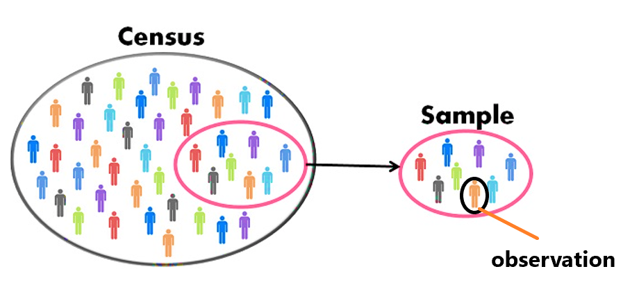
Can you tell me about population space or sample space?

Population space where all the observation are stored. Sample space is where some of the observation are stored. If your organization has 300K employees then the population space of all the employees of your organization is 300K. If you create a sample of 100 employees from this sample space then 100 employee are forming a sample space. Sample space is creating in sampling process. Every sampling has some purpose, therefore it must ensure that sample represents the population. There are many techniques to ensure this.

If there are 5 variables like Name, Age, Gender, Title, Salary then no two observations in the population or sample dataset can have the same information. Possible outcome of 2 observations in sample or population space can be “John Smith”, who is 35 years old, male, has a job title of “Manager”, and earns a salary of $ 70,000. Another possible outcome could be the employee named “Jane Doe”, who is 42 years old, female, has a job title of “Engineer”, and earns a salary of $80,000.

A sample space, often denoted by the symbol S, is the set of all possible outcomes of a random experiment. The population space, often denoted by the symbol Ω, is the set of all possible outcomes of a random process. The population space is typically not known and it is the sample space that we use to make inferences about the population.

What is Random Process, Random Experiment, Random Event, all are the same thing or different?

A random process is a sequence of events that cannot be predicted exactly. For example, tomorrow’s stock price of X stock. It depends on many dozens of variables.

A random experiment is an experiment in which the outcome is uncertain and can take on different values based on chance or probability. Traffic movement, dice throw, selecting employee, coin throw.

A random event is a specific outcome of a random process. Coming head in tossing random process, coming 4 in dice throw random process, selecting Ph.D holder from employee dataset, a vehicle can turn right on a traffic light.

What is the difference between variable and random variable?

An observation has attribute, for example an employee # 108 is one observation from our sample of population dataset. It has many attributes like name, age, gender, salary, position etc. These are variables. Any employee can have any value corresponding to these variables.

Random variable is a variable whose values are determined by a random process. For example if there can be only one job_position out of 4 job_position, then job_position variable is random variable. Output of random variables follows some distribution like normal distribution.

Every random variable is a variable but every variable is not a random variable.

What is the difference between Measure, Tool, Technique, Method, and Process?

• A measure is a way to calculate. It is a metric. For example mean, median, and mode are measures to know the central tendency of data. In our example dataset we can summarize the age column, as “mean age”=35 years, or median age is 38 years.
• A tool is a physical object or software or app used to accomplish a task. For example, Microsoft Project for creating a project schedule and identifying a critical path.
• A technique is a method or procedure used to accomplish a task. It is related to a simple problem. For example, a technique used to open the lid of an air-tight box or visualize 4 dimensional data on a 2D plane.
• A method is a systematic approach to solve a problem. It is more related to creativity and refers to a larger problem. For example, a method of cracking an IAS exam.
• A process is a series of steps or actions taken to achieve a desired result. For example the process of hiring.

What is the meaning of “sample” in statistics and how is it different from “observation”?

In statistics, a sample is a subset of a population that is chosen for the purpose of the study. A sample is a representation of the population. The goal of sampling is to select a group of individuals from a population that will be representative of the population as a whole. A sample is used to make inferences about the population from which it was drawn. A sample is used for estimating population parameters, such as the mean or standard deviation, and to test hypotheses about the population.

An observation, on the other hand, refers to a single measurement or data point. Observations are the individual pieces of data collected in a study. A sample can contain multiple observations, for example, a sample of 100 people means 100 different observations of different individuals, each observation can have multiple data points such as age, gender, income, etc.

In summary, a sample is a subset of a population, which is chosen to represent the population, while an observation is a single data point or measurement collected from an individual within the sample. A sample is used to make inferences about the population, whereas observations are used to make inferences about the sample.

What is the difference between statistics and census?

Statistics is the science of collecting, organizing, analyzing, and interpreting data. It is about sample data (a portion of the entire population).

Census is the process of collecting and counting data about a population. For example, to study the economic well-being of tribal people, if you can collect some sample data then it is part of statistics. But if you collect data on the entire tribal population then it is a census.

What are observational data, and experimental data in Statistics?

Observational Data: If you want to know whether there is any relationship between overtime working and number of defects produced then you collect the data and check the relationship. This collected data is observational data. Before collecting the data, we don’t have any intention of experimenting. We just want to know. To establish the relationship just observation of existing data is enough.

Experimental Data: If you change the number of working hours then what is the impact of this on number of defects produced? This way, you experiment with different working hours, sometimes you increase the hours, and at other times you decrease the hours. This collected data is experimental data. Before collecting the data I have an intention to experiment. In one experiment, we increased the number of working hours and then noted the number of defects. In another experiment, we decreased the number of working hours and then noted the number of defects. To establish this relationship you need to experiment multiple times.

Are statistical measures and statistical methods the same?

No, Statistical measures are the numerical values used to describe data, like mean, median, and standard deviation. While statistical methods are the techniques used to analyze data like regression, and statistical tests.

What are the different types of statistics?

The different types of statistics are

• Descriptive statistics
• Inferential statistics
• Predictive analytics.

What is Descriptive statistics?

Descriptive statistics is the process of summarizing and organizing data in order to describe the characteristics of a population or sample. It includes measures such as mean, median, mode, range, variance, standard deviation, quartiles, percentiles, skewness, kurtosis, and covariance. Each measure has a different formula to calculate. Apart from that, the same measure can be calculated differently for different data distributions.

What is Inferential statistics?

Inferential Statistics is a form of statistical analysis used to make inferences or draw conclusions from a given dataset. Generally, this involves testing assumptions and hypotheses about the data, such as if there is a relationship between two variables, or what the effect of one variable has on another. Inferential Statistics can help researchers to better understand the population they are studying.

What is predictive statistics?

Predictive Statistics is a branch of statistics used to make predictions about future events or outcomes. This is done by analyzing data sets and using mathematical models to uncover patterns and correlations that can be used to forecast potential results and trends. Predictive Statistics can be used in many different areas such as marketing, business forecasting, machine learning, and health care. Machine learning models are built for predictive statistics.

What are statistical measures of Descriptive Statistics?

Descriptive statistics measures include mean, median, mode, range, variance, standard deviation, quartiles, percentiles, skewness, kurtosis, and covariance. In statistics, we can study, and analyze these measures for sample data or for population data. In fact, when it is not possible to do a census then we use these measures of sample data and predict/extrapolate/postulate about the population measure. For example, if you want to know the average life expectancy of Indian women then you collect sample data and using that you can postulate about the average age of the entire indian women population. There is a process for doing this. In this process, there can be errors and there are processes of handling/factoring that error component.

What are statistical measures in Inferential Statistics?

Inferential statistics measures include z-score, t-test, chi-square test, correlation coefficient, confidence interval, and p-value.

What are statistical measures in Predictive Statistics?

To measure the performance of statistical models we have several measures. It depends upon the type of predictor or model type. For example, a classification model can be evaluated using precision, recall, accuracy, etc. A regression model can be evaluated using R^2 or Adjusted R^2.

What are the statistical tools in Inferential Statistics?

Inferential Statistics are statistical tools used to make inferences or draw conclusions from a given dataset. Examples of these tools include hypothesis testing, regression analysis, and correlation analysis. These tools allow researchers to infer information about population characteristics based on their observations of a smaller sample.

What are the statistical tools in Predictive Statistics?

Predictive statistics tools are machine learning algorithms, such as linear regression, logistic regression, decision trees, neural networks, and support vector machines.

About Variables & Models

What is a random variable?

• If you throw a die then the outcome can be any number between 1 to 6, inclusive.
• If you check the job applicant’s age then the age can be any number from 18 to 60, knowing this is the age limit.
• If you see traffic movement on a four-way cross junction it can be left, right, straight, or u-turn.

So the variables like dice-outcome, applicant-job, traffic-turn-direction can take any random value between the range or the options available. Therefore they are called random variables. In the language of the database, every table’s column is a random variable. In statistics, this is referred to as a random variable.

What are the different types of random variables?

A random variable can take any value from the given fixed number of options. For example, applicant_education applicant_gender, applicant_city, and dice_outcome can have a fixed number of outcomes. This kind of variable is called a categorical variable. Further, there are two types of categorical variables. Applicant_education can be Higher_Secondry, Graduate, Master, Ph.D. But this random variable has an order from low to high therefore it is called an ordinal categorical variable or ordinal variable. Applicant_city or color of the side of the die does not have any order therefore they are called nominal categorical variables or nominal variables.

In the employee dataset, what can be the value of applicant_age or salary? Like earlier, it is not selected from a fixed number of options available. Not only that it can be decimal also. Therefore such kind of random variable is called a numeric random variable or numeric variable.

Variable Types and Summarization

There are two kinds of variables and they are summarized in different ways.

• Summary of Nominal Variables: Count, Ratio, and Percentage, e.g. How many girls and boys, percentage of fruit tree vs no-fruit tree, percentage of bad product vs good product, etc.
• Summary of Numeric Data: mean, median, e.g. Mean salary, median age, mean sugar level, mean score
• Depending upon the situation, Ordinal data can be nominal or numeric.

Explain dependent variables and independent variables.

In regression, or in classification problems we want to predict or forecast something. It may be house-price, cost-of-project, time-to-complete-project, salary-of-new-hired, promotion of employee, churn-of-a-customer etc. These are called dependent variables. But to predict these we need the help of some other variables, on which the value of these dependent variables depends. Like house-price can be predicted from the area of a house, the cost-of-project can be predicted from the cost of the materials used, etc. These predictors are called independent variables. If there is only one predictor then we need simple linear regression. But in real business or personal life, you need more than one predictor, in that situation multi-linear regression is needed to predict.

What is the difference between the regression coefficient and correlation coefficient?

The regression coefficient is used to quantify the relationship between two variables. It can tell you keep all variables constant if you change a variable (related to regression coefficient) by 1 unit then how much change will happen on the target variable. The regression coefficient takes into account the slopes and intercepts of the line of best fit that is created when plotting the data points. The regression coefficient also allows for a more accurate prediction of outcome values based on input values.

While the correlation coefficient measures the direction and strength of the linear relationship between two variables.

What is a statistical model?

A statistical model is a mathematical representation of a real-world phenomenon. It is used to make predictions and analyze data. The data generated by the model and real-world data will have some differences and this is called an error in the model. For example, based on certain parameters like carpet_area, number_of_bedroom, etc. a model can predict house price should be 1.2 crores, but the actual price is 1 core. Thus, the model is predicting the price as 20 lakhs Rupees more. This is a model error. Keeping people’s behavior, market opportunities, etc in mind we can never make a statistical model with zero error. But if I could guess the distribution of input variables correctly then the output of our model will have fewer errors.

What is the difference between Statistical Model and Mathematical Model?

Mathematical models are deterministic, the input is clearly known, the outcome is fixed. Newton’s equation of motion is a Mathematical Model. It represents the physical reality of the world. In \(s = u*t + \frac{1}{2}*a*t^2\) You provide the value of u,t, and a and you will get accurate s.

Statistical models are non-deterministic or stochastic, some of the inputs are probabilistic, and the outcome is also probabilistic. When you develop a model to predict a house price then you need a statistical model. In your model parameters may be carpet_area, number of bedrooms, etc. From the sample data, we know if the area is 2000sft then the price can be 1cr, it can be 1.2cr, or 1.5cr. For the same carpet area the price is different. It is not only because of other parameters but because of market opportunities. Thus input and output of the model will be probabilistic. Because of this non-deterministic nature, we need to assume the distribution of the data, so that outcome is more certain.

About Tools & Techniques

What is regression?

If you want to predict salary from experience or the “number of projects done” then you can use regression analysis.

A generic linear regression equation is \(y=mx+c\). Where y is a dependent variable like salary (which you want to predict), x is an independent variable like no_of_years_experience. m is the slope of the line or coefficient. c is an intercept of the line, which will give you the value of salary even if the experience is zero. For example, this model will predict salary in lakhs. \(Salary=2.5*no\_of\_years\_experience+1\)

What is Correlation and What is the formula of this?

When you want to know the strength and degree of relationship between two variables you can you Correlation measure. Its value ranges between -1 to 1. 0 correlation coefficient means there is no relationship between two variables and they move randomly with respect to each other. Negative correlation means they move in the opposite direction, when one increases the other decreases and vice versa. Positive correlation means they move in the same direction, when one increases the other also increases and vice versa. When two variables are numeric you can use Pearson correlation.

The formula for Pearson’s correlation coefficient, denoted by “r,” is:

\[r = \frac{\sum_{i=1}^{n}(x_i - \bar{x})(y_i - \bar{y})}{\sqrt{\sum_{i=1}^{n}(x_i - \bar{x})^2} \sqrt{\sum_{i=1}^{n}(y_i - \bar{y})^2}}\]

you can also write it like

\[r = \frac{ \frac{\sum_{i=1}^{n}(x_i - \bar{x})(y_i - \bar{y})}{n} } {\sqrt{ \frac{1}{n}\sum_{i=1}^{n}(x_i - \bar{x})^2} \sqrt{ \frac{1}{n} \sum_{i=1}^{n}(y_i - \bar{y})^2}}\]

or

\[\rho_{(x,y)} = \frac { Cov(x, y)} {(Std(x) * Std(y)) }\]

where x and y are the two numeric variables being correlated, n is the number of observations, and $\bar{x}$ and $\bar{y}$ are the means of the x and y variables, respectively.

How many types of correlation coefficient are there in stats?

There are several types of correlation coefficients that are commonly used in statistics to measure the strength and direction of a linear relationship between two variables. Here are a few of the most common ones:

1. Pearson correlation coefficient: The Pearson correlation coefficient is a measure of the linear relationship between two variables. It ranges from -1 to 1, where -1 indicates a strong negative relationship, 0 indicates no relationship, and 1 indicates a strong positive relationship. For example: relationship between experience and salary.

2. Spearman rank correlation coefficient: The Spearman rank correlation coefficient is a nonparametric measure of the strength of the monotonic relationship between two categorical variables. It is calculated based on the ranks of the values rather than the raw data. For example: relationship between gender and bone cancer.

3. Kendall rank correlation coefficient: The Kendall rank correlation coefficient is another nonparametric measure of the strength of the monotonic relationship between two variables. It is calculated based on the number of concordant and discordant pairs in the data.

4. Partial correlation coefficient: The partial correlation coefficient is a measure of the correlation between two variables, taking into account the influence of one or more additional variables.

5. Intraclass correlation coefficient: The intraclass correlation coefficient is a measure of the degree of agreement between observations that are made on the same subjects. It is commonly used in the analysis of repeated measures data.

It’s important to choose the appropriate correlation coefficient based on the nature of the data and the type of relationship you are interested in.

What is AutoCorrelation?

Let’s say we have share price data of a company. These observations are monthly. We want to know if there is any pattern in this monthly data? For that purpose we try the relationship between the stock price. But this time the original stock price is associated with “after month share price”. This shifting is called one month lagging, it means 1949-01 data is compared with 1949-02 data, and so on. Similarly you can shift data 2 time periods or 3 time periods. When you check the relationship between original share price and 1 lagged shared price or 2 lagged shared price or 3 lagged share price it gives you a correlation coefficient. This process is called AutoCorrelation. Whatever number of month’s shifts shows higher correlation, that number of months is interesting for us.

Mean=>	127		128	127
Month	Passengers (y)	\(y_{t-1}\)	\(y_{t-2}\)	\(y_{t-3}\)
1949-01	112
1949-02	118	112
1949-03	132	118	112
1949-04	129	132	118	112
1949-05	121	129	132	118
1949-06	135	121	129	132
1949-07	148	135	121	129
1949-08	148	148	135	121
1949-09	136	148	148	135
1949-10	119	136	148	148
1949-11	104	119	136	148
1949-12	118	104	119	136
1950-01	115	118	104	119
1950-02	126	115	118	104

What is the AutoCorrelation formula?

The AutoCorrelation formula is the same as the Correlation formula. Only difference is Y is taken from the time lag of X.

\(\rho_{X_t, X_{t+\tau}} = \frac{\displaystyle \sum_{t=1}^T (X_t - \overline{X})(X_{t+\tau} - \overline{X})}{\displaystyle \sum_{t=1}^T (X_t - \overline{X})^2}\),

where \(\bar{X}\) is the mean of the data set X, \(\tau\) is the lag, and T is the length of the data set.

Causation and Correlations are two different things, can you explain them with an example?

Causation means that a change in one thing causes a change in another, while correlation means that two things occur together without necessarily being connected. Let’s see examples:

1. Studies have shown that there is a positive correlation between the amount of time spent studying and good grades, but this does not necessarily mean that studying causes good grades. It could be that other factors such as access to excellent teachers, resources, and tutors cause both studying and good grades.
2. There is a positive correlation between smoking and lung cancer. However, this doesn’t necessarily mean that smoking causes lung cancer. Other factors such as genetics, lifestyle, and environment may also play a role in developing lung cancer.
3. There is a positive correlation between exercising and improved physical health, but this doesn’t necessarily mean that exercising causes improved physical health. Other factors such as diet, sleep, and genetics may also play a role in physical health.
4. There is a positive correlation between eating junk food and becoming overweight, yet this doesn’t necessarily mean that junk food causes overweight. Other factors like exercise, genetics, and stress levels can also contribute to weight gain.
5. There is a positive correlation between drinking alcohol and developing liver disease, yet this doesn’t necessarily mean that drinking alcohol causes liver disease. Other factors such as genetics, lifestyle, and environment may also be contributing factors.

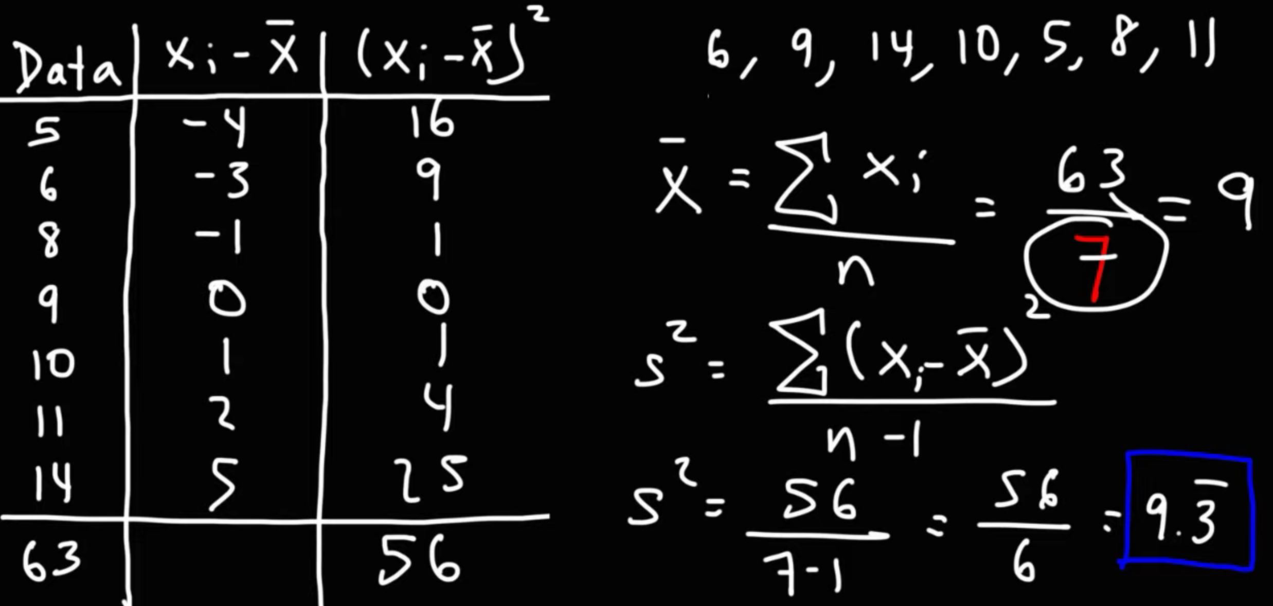
What is Variance and how to calculate variance?

If your dataset has a column “Age” and all people are 25 years, it means the variance of the Age column is zero. From an analysis and model-building perspective this column is useless. Only those columns, which have some variance are useful, the more the variance the better is the column.

Variance is a measure of the dispersion of a single column of data. It is calculated as the sum of the “squared differences” between each “data point” and the “mean of the data”, divided by the number of data points.

Variance of population dataset is calculated as below. \(\sigma^2 = \frac{\sum_{i=1}^{n} (x_i - \mu)^2}{n}\)

Variance of the sample dataset is calculated as follows. \(\sigma^2 = \frac{\sum_{i=1}^{n} (x_i - \mu)^2}{n-1}\)

Are correlation and regression different or same thing?

If you want to study the magnitude or direction of the relationship between two variables you can use correlation statistical measure.

Regression analysis is a statistical technique used to analyze the relationship between two or more variables. It can also help in prediction.

What is Covariance and how to calculate it?

The idea behind variance and covariance is the same. The only difference is in variance we check the variation of one column from it means, but in covariance we check how closely two different variables walk together.

Let’s assume your dataset has 2 columns, age, and experience. We want to know the relationship between these two columns, for this we can calculate covariance, how strongly two column values move together. They can move in the same direction or in the opposite direction. A higher absolute value means two columns are moving strongly with each other.

It is calculated as the sum of the “products of the differences” between each “data point in one set” and the “mean of that set”, and the differences between the corresponding data points in the other set and the mean of that set, divided by the number of data points.

\[cov(X, Y) = \frac{\sum_{i=1}^{n} (x_i - \mu_X)(y_i - \mu_Y)}{n}\]

What is the AutoCovariance Function (ACVF) Formula?

Mean=>	127		128	127				AutoCovariance 16	AutoCovariance -51
Month	Passengers (y)	\(y_{t-1}\)	\(y_{t-2}\)	\(y_{t-3}\)	\(y_t - \bar{y_t}\)	\(y_{t-2} - \bar{y}_{t-2}\)	\(y_{t-3} - \bar{y}_{t-3}\)	(\(y_t - \bar{y_t}\)) * (\(y_{t-2} - \bar{y}_{t-2}\))	(\(y_t - \bar{y_t}\)) * (\(y_{t-3} - \bar{y}_{t-3}\))
1949-01	112
1949-02	118	112
1949-03	132	118	112
1949-04	129	132	118	112	2	-9	-15	-18	-30
1949-05	121	129	132	118	-6	5	-9	-30	54
1949-06	135	121	129	132	8	2	5	16	40
1949-07	148	135	121	129	21	-6	2	-126	42
1949-08	148	148	135	121	21	8	-6	168	-126
1949-09	136	148	148	135	9	21	8	189	72
1949-10	119	136	148	148	-8	21	21	-168	-168
1949-11	104	119	136	148	-23	9	21	-207	-483
1949-12	118	104	119	136	-9	-8	9	72	-81
1950-01	115	118	104	119	-12	-23	-8	276	96
1950-02	126	115	118	104	-1	-9	-23	9	23

AutoCovariance is the same as variance. The only difference is you are not checking the relation between two different columns but the same column’s value with different time lag. It is used in timeseries data. Let’s assume your dataset has a 365 day’s closing price of TCS. If you want to know how much the price of today is related to the price of last week then you can AutoCovariance.

AutoCovariance formula is

\[\gamma(k) = Cov(X_t, X_{t+k})\]

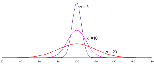
What is Standard Deviation and what is the formula to calculate this?

Standard Deviation (SD) is a measure of spread or dispersion around the mean. It is also called Sigma and written as \(\sigma\). It quantifies the amount of variation or dispersion of a set of data values. For any data column larger the value of means more the spread. The standard deviation is the square root of the variance. Larger value indicates a more flatten normal distribution.

The formula for the “sample standard deviation”, denoted by “s,” is:

\(s = \sqrt{\frac{1}{n-1}\sum_{i=1}^{n}(x_i - \bar{x})^2}\) OR

\[s = \sqrt{Sample\_Variance}\]

where x is the set of observations, n is the number of observations, and $\bar{x}$ is the mean of the observations.

The formula for the population standard deviation, denoted by “σ,” is:

\(σ = \sqrt{\frac{1}{n}\sum_{i=1}^{n}(x_i - \mu)^2}\) OR \(σ = \sqrt{Population\_Variance}\)

where x is the set of observations, n is the number of observations, and $\mu$ is the mean of the observations.

What is standard scaling or z score calculation?

Standard scaling of a numeric column means converting normal values into z scale values. Let’s say our salary column minimum value 20,000, maximum value 150,000 and mean value 50,000. If this column is normally distributed then 50% of the people will have a salary <=50,000 and 50% of the people will have a salary >50,000. When you convert this column into z-scale you need to calculate the z-score of every value. In that situation the z-value of the mean will become 0, and less than mean values will become negative z-values and more than mean values will become positive z-values. After this scaling you can say 99% of the data is within -3 to +3 Z scale. You can pick-up any other column, like age, which is a completely different scale compared to salary. When you convert that into z-scale then 99% of the age will be within -3 to +3 z scale. For calculating z score we can use the formula \(\frac{X-\mu}{\sigma}\). This is called standard scaling of salary column values.

Thus a z-score is a description of how far a sample or point of data is away from its mean. Z score value can be negative or positive. Larger the absolute z score value of any point, far away that is from the mean. For example, if we want to calculate the z-score of a salary 30,000 then the Z score of 30,000 = (30,000 - 50,000) /10,000 = -2. It means a 30,000 salary is 2 distance away from the mean, but left side.

If we want to convert a salary of 70,000 into sigma value we get z score = (70,000-50,000)/10,000 = 2. It means a 70,000 salary is also 2 distance away from the mean but right side.

During a statistical test we need to make sure that z score of any given value should not fall in the critical range, otherwise the null hypothesis will be rejected. We will discuss this in detail at another place.

Because of its utility and applications, In statistics and process control perhaps Sigma or SD or Standard Deviation is the most popular measure.

Sigma of Statistics, Sigma of process control and Z score are confusing and sometimes used interchangeably.

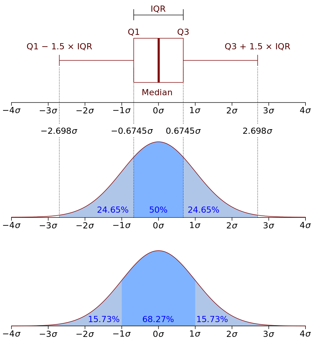
What is the Sigma value in Statistics (Normal Distribution)?

It helps us in understanding the distribution of sample data. It helps us in knowing the probability. If 1 Sigma is 10,000, then 68% samples will have a salary between mean_salary \(\pm 10000\).

Sigma Level	Confidence	Significance	Area on the edge of curve
\(\pm 1 \sigma\)	68.00%	34.00%	34% left or 34% right or 17% left and 17% right
\(\pm 1.64 \sigma\)	90.00%	10.00%	10% left or 10% right or 5% left and 5% right
\(\pm 2 \sigma\)	95.00%	5.00%	5% left or 5% right or 2.5% left and 2.5% right
\(\pm 3 \sigma\)	99.00%	1.00%	1% left or 1% right or 0.5% left and 0.5% right

What is Sigma value in Process Control?

It helps us see how much maximum error a process can do. If a packing process is 5 sigma then it will not make more than 233 packing errors out of 1 million packings.

Sigma Level	Defects/Mn Opportunities or DPMO	Yield	Defects in %	Yield %	9s
1	691462	308500	69.1462	30.85	0 9s
2	308538	691460	30.8538	69.146	0 9s
3	66807	933190	6.6807	93.319	1 9s
4	6210	993790	0.621	99.379	2 9s
5	233	999767	0.0233	99.9767	3 9s
6	3.4	999997	0.00034	99.9997	5 9s

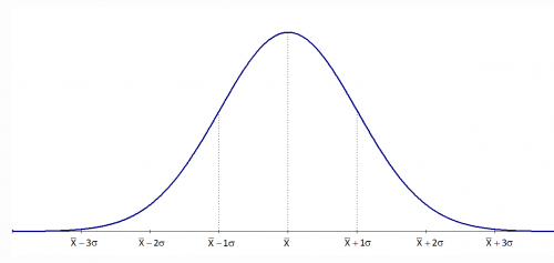
What is the meaning of Standard Deviation (SD) of the sampling distribution of the mean?

What is Sample Standard Error OR Standard Error of Sample Mean?

The SD of the sampling distribution of the mean, also known as the “standard error (SE) of the sample mean”. It is a measure of the variability of the sample mean. It is used to estimate the precision of the sample mean as an estimate of the population mean.

To understand this concept, let’s consider an example. Imagine you are studying the heights of adult males in a certain population. The population mean height is 170 cm and the population standard deviation is 10 cm. If you take a sample of 5 adult males, you would calculate the sample mean height. Each time you take a different sample of 5 adult males, you would get a different sample mean height.

Now, imagine taking many samples of 5 adult males, each time calculating the “sample mean height”. The distribution of the “sample mean heights” is known as the “sampling distribution of the mean”. The SD of this “sampling distribution of the mean” is called the “standard deviation of the sampling distribution of the mean” or the “standard error of the sample mean”.

In other words, the “standard deviation of the sampling distribution of the mean” is a measure of the variability of the sample mean. It tells us how much the sample mean is likely to deviate from the population mean, given a certain sample size. The smaller the “standard deviation of the sampling distribution of the mean”, the more precise the sample mean is as an estimate of the population mean. This means, as the sample size increases, the “standard deviation of the sampling distribution of the mean” decreases, the sample mean becomes a more accurate estimate of the population mean.

\[SE = \frac{s}{\sqrt{n}}\]

SE is the Standard Error,
s is the standard deviation of the sample
n is the sample size

In our dataset if the salary column has mean_slary=50,000 then we know some observations will have less than 50K and others will have more than 50K. If we do the total of this difference between actual_salary and mean_salary we will get standard error. \(SE = \frac{X-\bar{X}}{n}\).

If you don’t know this \(X-\bar{X}\) but you know s then you can calculate it like following \(SE = \frac{s}{\sqrt{n}}\)

If you know the variance but not SD then you can calculate as following \(SE = \frac{ {\sqrt{variance}}}{\sqrt{n}} = \sqrt{\frac{variance}{n}}\)

What is Population Standard Error OR Standard Error of Population Mean?

In statistics, the standard error of the population mean, denoted as σM or σ/√N, is a measure of the variability of the population mean. It is the standard deviation of the sampling distribution of the population mean. It is used to estimate the precision of the population mean, but it is not commonly used because often the population standard deviation and population size are not known.

The standard error of the population mean is based on the assumption that the population is normally distributed. If the population is not normally distributed, the standard error of the population mean cannot be calculated and other methods must be used to estimate the precision of the population mean.

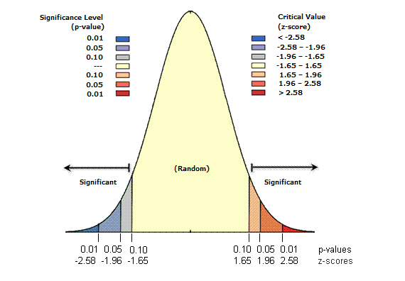
How to use z score for probability calculation?

z-score (Standard Deviations)	p-value (Probability)	Confidence level
< -1.65 or > +1.65	< 0.10	90%
< -1.96 or > +1.96	< 0.05	95%
< -2.58 or > +2.58	< 0.01	99%

If the mean salary in our dataset is 75,000 and SD is 5000 then what is the probability that the salary of a randomly chosen employee is >90,000

Method1 You can get z score of this 90,000
\(z = \frac{x - \mu}{\sigma}\) = (90000 - 75000) / 5000 = 3
Pr for Z<=3 (salary <= than 90K) => .99865
Pr for Z>3 (salary more than 90K) => 1-.99865 = .00145

Above z values we can get from z-table. Z tables are based on standard deviation of normally distributed data. Z table gives probability values for a given z score or standard deviation (SD). If data is not normally distributed then you will not get correct probabilities.

Method2 You can put these values in a normal distribution formula and you will get the same value.

\[\varphi(x) = \frac{1}{ \sqrt(2\pi\sigma^2)}*e^\frac{ -(x-\mu)^2}{2\sigma^2}\]

What is the Box-Cox Normality Plot?

Many statistical tests and intervals are based on the assumption of normality. The assumption of normality often leads to tests that are simple, mathematically tractable, and powerful compared to tests that do not make the normality assumption. Unfortunately, many real data sets are in fact not approximately normal.

The Box-Cox transformation is a particularly useful family of transformations. It is defined as:

\(T(Y) = (Y^{\lambda} - 1)/\lambda \qquad (\forall \lambda>0)\) \(T(Y) = ln(Y) \qquad (\forall \lambda=0)\)

What is skewness?

Skewness measures the lack of symmetry in a data distribution. It indicates that there are significant differences between the mean, the mode, and the median of data. If you want to use skewed data for modeling or analysis purposes then you need to transform this into a normal distribution. The curve below is left skewed.

\[skewness = \frac{\sum_{i=i}^{n}{({x_i - \bar{x}}})^3}{(N-1)*\sigma^3}\]

Right skewed = Positive Skewed
Left skewed = Negative Skewed

What is kurtosis?

Kurtosis is a measure of the “tailedness” of the probability distribution of a real-valued random variable. The long tail will have kurtosis.

\[kurtosis = \frac{\sum_{i=1}^n{({x_i - \bar{x}}})^4}{var^2}\]

What is the R-Square formula?

R-Square or $R^2$ is also called the coefficient of determination. It is used to evaluate the performance of the regression model. $R^2$ value can be any number between 0 and 1 including 0 and 1. It can never be negative. If $R^2$ of a model is .80 then it means this model explains 80% variation between actual and predicted values but 20% variation cannot be explained. A higher $R^2$ value means more variation can be explained by the model and better the model is.

\[R^2 = 1 - \frac{SS_{res}}{SS_{tot}}\]

Where \(SS_{res}\) is the sum of squared residuals (the difference between the predicted value and the actual value) and \(SS_{tot}\) is the total sum of squares (the difference between the actual value and the mean of all actual values).

What is the Adjusted R-Square formula?

It is used to understand whether any newly added feature is adding any value to the model or not. Because this model adds a penalty for every newly added variable, therefore if the addition of a new variable in the model does not increase R^2 more than the penalty added then overall R^2, adjusted R^2 will decrease.

\[Adjusted R^2 = 1 - (1 - R^2) * \frac{(n - 1)}{(n - p - 1)}\]

About Probability & Distributions

What is probability?

A ratio between “chances of getting success” and number of outcomes available.

A die has 6 faces, if success = coming 4 success on top, then the chances of getting 4, the success=1. Total number of outcomes (1,2,3,4,5,6)=6. Probability of getting success 1/6

What is log-odd?

It is also called logit. It is used more in logistic regression. It is a log of the odds.

An odd is a ratio between “chances in favor” and “chances against”. When you throw a fair coin, total chances are 2 (head, tail). If success means head come then chances of coming head is 1, chances of tail come is also 1. In this case the odds of head coming or success is 1.

\[logodd(event=success) = log( \frac{p}{(1-p)})\] \[p(event=success) = 1/2 = 0.5\] \[logodd(event=success) = log( \frac{p}{(1-p)}) = log(\frac{.5}{1-.5}) = log(1) = 0\]

It is important to note that the log-odd of getting a head is zero only when the coin is fair, if the coin is not fair, the log-odd will be different.

What is the difference between theoretical probability and experimental probability?

Success probability of all the outcomes may not be the same. This you can know from historical data. For example, if you go to your friend’s house without calling him, what is the probability you will find him at home? ½ or 50%. This is theoretical probability. But from your past experience you know out of 50 times he was available only 5 times. So success probability (experimental probability) your friend is at home is 5/50 = 1/10 = .1 = 10%.

Similarly in die through game theoretical probability of getting 2 is ⅙. But if die is tampored in the favor of 2 then the probability of getting is more than ⅙ or probability of getting any other number is less than ⅙.

If the stock-market opens today then will the share price of Infosys go up, or down or remain as it was on the last day? Theoretical probability of opening at a higher price is ⅓. But from historical data you may know the market is in favor or against Infosys at the start of day.

What is success probability?

Let’s assume our job_applicant dataset can have applicants only from 6 cities (Mumbai, Delhi, Bangalore, Chennai, Hyderabad, and Kolkata). In this dataset, you have 10,000 applicants’ information. Now if you are interested in only those employees who are from Mumbai, then you can ask questions like, what is the probability that a given employee is from Mumbai? In the experiment, if you pick up record number 1008 and this candidate is from Mumbai then you call the event successful. But, if the candidate is from any other city then, you call the event a failure. You write it as \(Pr(Applicant\_city=Mumbai)\).

If this dataset has 2000 candidates from Mumbai then a randomly selected candidate will be from Mumbai, what is the probability? 2,000/10,000 = .20 or 20% so \(Pr(Applicant\_City=Mumbai)=.20\). 20% is the success probability.

Success probability is a little tricky in the case of a numeric variable. Because if you want to check the probability of a person whose age is 35 years, 3 months, 10 days, and 6 hours then the question is valid but the answer is Probability of success of this event is zero. You pick up any number and the answer is going to be like that. For example, when you say age is 30 years, it means 30 years, 0 months, 0 days, and 0 hours. Due to this reason with numeric probability you either use >= or <=. It means you can ask a question like, what is the probability of Age of a candidate [<=30, or >=30], or [>=30 but <=35] years?

In our dataset, if we have 3000 people who are <= 30 years then Pr(Applicant_Age<=30) = .30 or 30%.

If our dataset has 5000 people <=35 years then \(Pr(Applicant\_Age<=35) = .50\) or 50%.

Now we can say Pr(Applicant_age>=30 and <=35) = .50 - .30 = .20 or 20%.

This all is done by exploring another concept called probability density.

What is probability density?

Let’s assume our dataset has 10,000 applicants and their age is between 18 to 60 years. You can plot a histogram and this histogram represents the distribution of age of the applicants. The entire area of this histogram is referred to as 1, in our case 10,000 people’s age is represented by this area and it is 1. This is the total density of this curve. The X-axis of this curve will have age and the Y- axis will have a number of people.

Shapes of Various Distributions

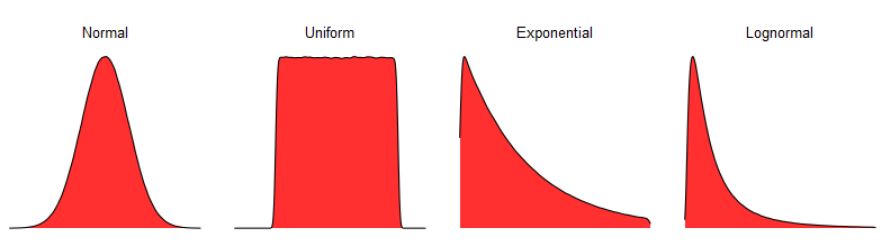
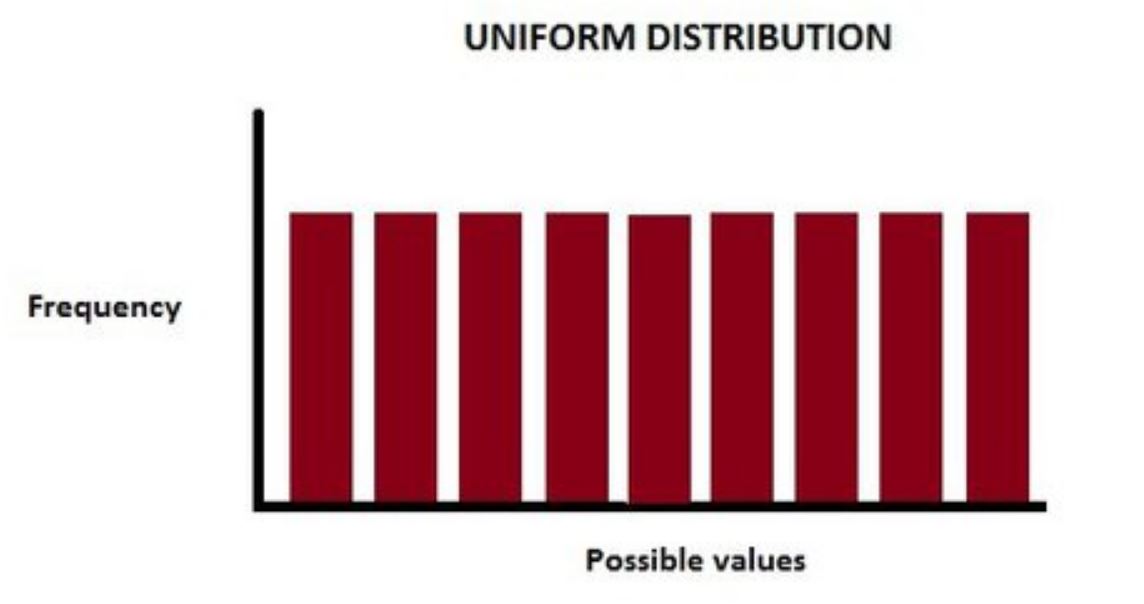
What is uniform distribution?

Suppose in our dataset, if the number of people in each age group of 10 years like 18-28, 28-38, 38-48, etc we have an equal number of people then it is a uniform distribution..

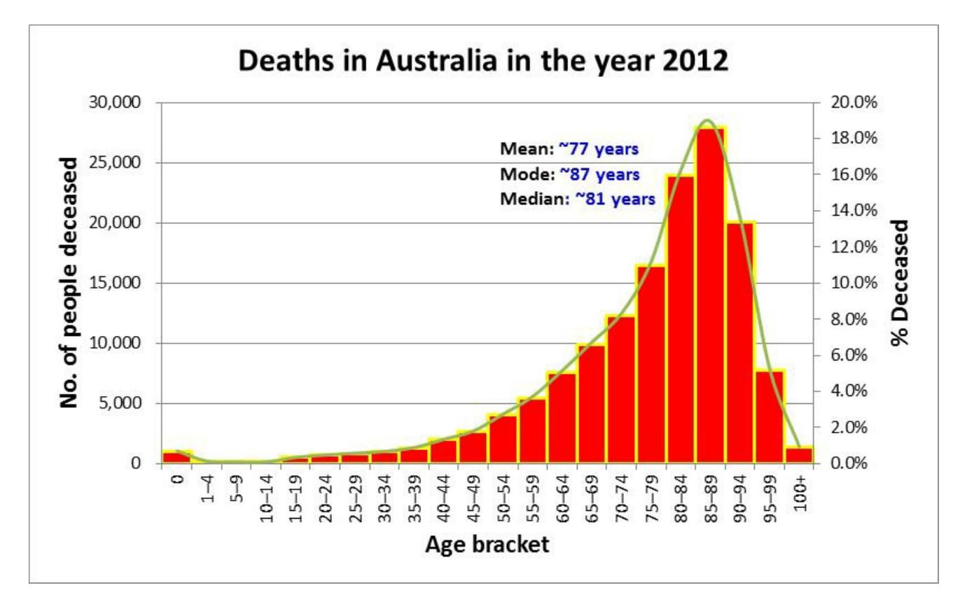
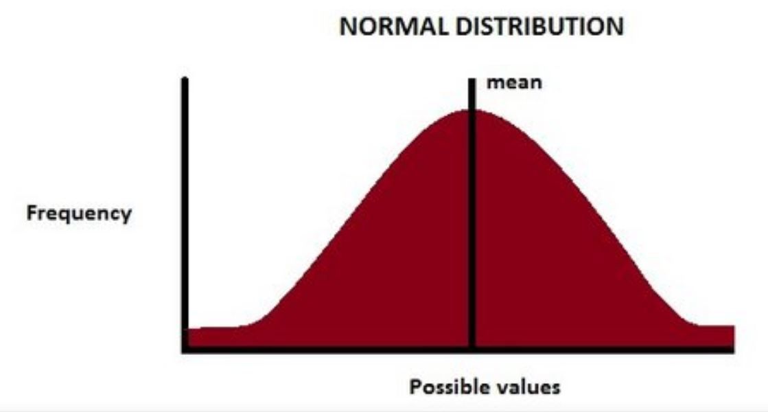
What is a normal distribution? What is the use of this?

In our dataset, the minimum age is 18 years (recently hired), but there are fewer people like this. The maximum age in the dataset is 60 years (people are going to retire this year), but there are fewer people like this. If you plot the histogram of this “age” information you will get a normal distribution. It is also called Gaussian distribution, It means the mean and median will be 40 years, 5000 employees are <= 40 years old and 5000 employees are > 40 year age.

If this age data is truly normally distributed then 68% of employees will be within \(\pm 1\sigma\), 95% of employees will be within \(\pm 2\sigma\), and 99% of employees will be within \(\pm 3\sigma\).

Characteristics of Normal Distribution

• Curve is a perfect bell curve (Unimodal, only one peak). Due to this reason, the normal distribution curve is also called the bell curve.
• Mean=Median=Mode
• Area less than mean = 0.5, and the area more than mean = 0.5 (symmetric)
• Asymptotic on both sides of the curve

Formula to calculate the probability of a random variable having a normal distribution. \(\varphi(x) = \frac{1}{ \sqrt(2\pi\sigma^2)}*e^\frac{ -(x-\mu)^2}{2\sigma^2}\)

Examples : The height of people, the weight of people, IQ scores, blood pressure levels, grades on a test, marks on a sports field, finger lengths, frequency of letters in a language, errors in a manufacturing process, and the time it takes for a web page to load

Source: Wikipedia

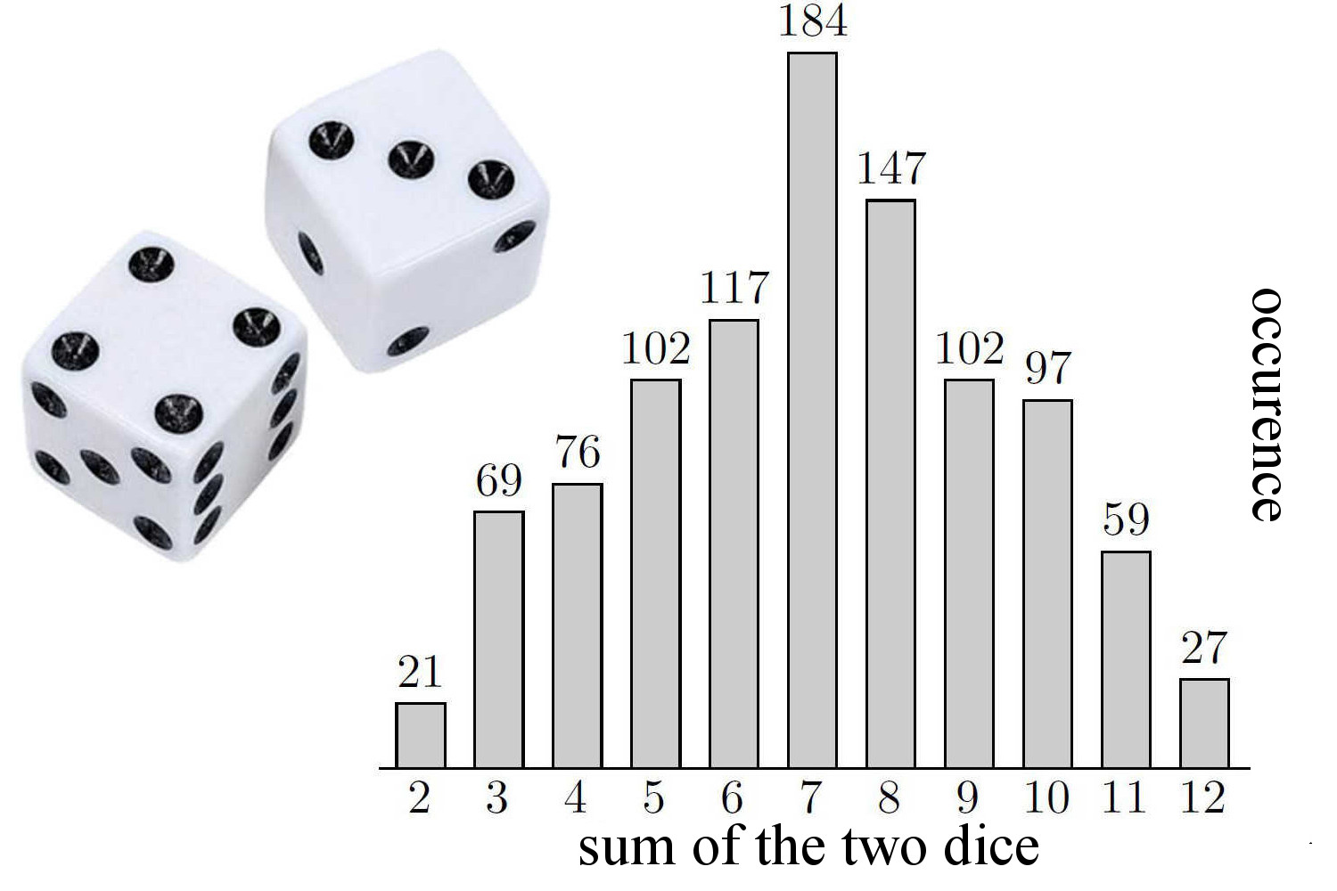
What is binomial distribution? What is the use of this?

If you throw 2 dice simultaneously then the sum of the outcomes can be anything between 2 to 12.

First Dice	1	2	3	4	5	6
Second Dice
1	2	3	4	5	6	7
2	3	4	5	6	7	8
3	4	5	6	7	8	9
4	5	6	7	8	9	10
5	6	7	8	9	10	11
6	7	8	9	10	11	12

There are a total 36 ways (above combinations) to get any number between 2 to 12. There is only one way to get 2, 2 ways to get 3, 3 ways to get 4, 4 ways to get 5, etc.

So the probability of coming 10 is 3/36, the probability of coming 7 is 6/36 = 1/6, etc. The probability of coming 7 is the highest.

If you throw these two dice together 100 times then what is the probability 20 times the total sum of 7 will come? To get this answer you need a distribution formula, a distribution that determines this whole game.

This whole game can be predicted using the binomial distribution. Formula is \(pr(success=r\, times)= nC_rP^r(1-P)^{n-r}\), where n= number of times experiment repeated, r=number of times success happens, p=probability a success happens. The probability of success means the probability of getting 7. for p=1/6. \(pr(success=20 \,times \, total \, is \, 7)= 100C_{20}\frac{1}{6}^{20}(1-\frac{1}{6})^{100-20} = 0.0678\)

We can use binomial distribution for any experiments where the outcome is either success or fail (binary) and experiments n times and we want to know the success for r times.

Application: You are tracking the stock price for TCS shares for the last 500 days. You want to know that in the next 100 days, the probability of the stock price will cross Rs 800, 10 times.

You can get the P value, the probability of success from 500 days of data. Let’s say it has crossed 800, 40 times. P=40/800 = .05.

\[pr(success=10 \,times)= 100C_{10}\frac{1}{.05}^{10}(1-.95)^{100-10} = .0.0167\]

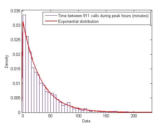
Can you give example of exponential distribution

Where time is on X axis

• Time between arrivals of customers to a store,
• Time between arrivals of cars at an intersection,
• Time taken by the computer system to respond to user requests.
• Over a period of time the amount of money spent on goods and services,
• Over a period of time number of mutations in a gene sequence,
• Number of web pages visited over a given period.
• Over a period of time the number of deaths due to a particular disease.
• Over a period of time radiation levels of radioactive materials,
• Over a period of time the length of time it takes for a user to complete a task
• The amount of radioactive material decayed over a given period

Where time is NOT on X axis

• Size of earthquakes, the length of coastline
• Size of earthquakes, and number of casualties
• Number of time compression and the size of a computer file after compression
• Distance and the intensity of light from a star.

Exponential Distribution

About Hypothesis Testing

What is p-value?

P value is the probability in the favor of the null hypothesis. It is used to evaluate the hypothesis.

• Higher p-value means it is supporting H0.
• Higher p-value means it is against H1.
• Lower p-value means it is supporting H1.
• Lower p-value means it is supporting H0.

You can read the p-value from the z-table. It means, if you know the z value of any observation you can know the p-value of that.

For example: if we want to know what is the probability that someone has a salary <=40000 we can calculate the z score of 40,000 and read the p-value of that z-score from the z-table.

What is the Significance Level?

Total Probability = Confidence Level + Significance Level. If confidence level is 95% then significance level is 5%. If confidence level is 99% then significance level is 1%.

Significance level means margin of error. Error means when you predict incorrectly, or opposite of ground truth. If you predict it will rain, but it doesn’t rain this is called an error. If you predict it will not rain, but it rains, this is also called an error.

What is Type-I and Type-II error?

Type-I error is when H0 is wrongly rejected. It is also called false positive. Type-II error is when H0 is wrongly accepted. It is also called false negative.

If a good tweet is blocked by twitter then it is Type I error. If a good product is wrongly rejected by the quality team, it is Type-I error. If an innocent person is fined by the income tax department, it is Type-I error. If a healthy person is wrongly detected as infected, it is Type-I error.

If an offensive or hateful tweet is blue ticked by twitter then it is type II error. If a bad product is wrongly accepted by the quality team it is Type-II error. If a tax invader is not fined by the income tax department, it is Type-II error. If an infected person is wrongly certified as a healthy person, it is Type-II error.

How to select the right Statistical Test for a problem in hand?

In the process of statistical testing, choosing a correct statistical test is a very important step. Which test is applicable for the problem can be determined using the following.

1- What kind of data we have (numerical or categorical)
2- How many samples we have (1, 2 or many). Each sample has dozens or hundreds of observations.
3- How many variables we have (1 or 2). Like age, temperature, sale, number of people etc.
4- Whether variables are paired for each observation or not.

• Example of pair can be, salary and experience of the same person. Blood sugar of the same person, before fasting, then post fasting. It is 2 variable and 1 sample.
• Examples of unpaired, two groups, one have gone through meditation and another have not gone through meditation. We check their BP after 15 days. It is one variable but 2 samples.

5- Purpose of test. We want to compare two sample mean/median etc, or we want to compare sample mean with population mean, or we want to check relationship between two variable

Selecting a correct statistical test for a given scenario is very challenging task for most of the non-statistics background people

Statistical Tests with Example

• CASE1: Mileage claim: An automobile manufacturing company claims their car’s average mileage is 20 Km/Liter. Automobile Association collects data of 100 automobiles, calculating the mean as 19 KM/Liter, SD=.5. Now they can compare this sample mean with population mean (20 km/liter). Whether the automanufacture’s claim is valid, at 5% significance level?
  SOLUTION: Data- Milage (Numeric).
  Sample: 1 sample, we need to compare the mean with population mean.
  Purpose: Compare the data against the population claim.
  H0: Mu mileage >= 20 km/liter or Mu consumption <= 50ml/km
  H1: Mu mileage < 20 km/liter or Mu consumption > 50ml/km
  Test: Test of Mean or t-Test. Z-Test SE = s/sqrt(n) = .5/10 = .05 z = (x - mu)/SE = (19-20)/.05 = -20, z score for critical value 5% is -1.96. The Z-score of of the sample mean is extremely less than critical value, therefore the H0 is rejected.

• CASE2: School-Leavers and Working Duration: Whether school leavers tend to stay a longer or shorter time in the company than people who have worked elsewhere first. HR collects the data of 100 ex employees, their number of years stay and joining information. They summarize the data as follows: mean stay time of joinee from school= 8 years, mean stay time of joinee from other company is 7.5 years. Now you can compare these two. Whether there is any relationship between how long people will work and from where they join?
  SOLUTION: Data - Stay Duration (numeric)
  Sample : 2 sample unpaired (school leaver vs other)
  Purpose: Compare the mean of two groups.
  H0: Mu School Leavers = Mu Others
  H1: Mu School Leavers <> Mu Others
  Test: Difference of 2 Means (independent samples). t-Test

• CASE3: Defect Claim: An electronics manufacturer does not allow more than 1% fault on their components. The quality manager gets data of 500 components and finds 11 are faulty. Whether the company is working as per the standard set by them?
  SOLUTION: Data- Faulty or Non Faulty (Nominal Data)
  Sample: 1 sample
  Purpose: Compare against the standard.
  H0: Defects <= .01
  H1: Defects > .01
  Test: Test of Proportion. Z-test

• CASE4: Recruitment Assessment: Recruiter gives you a test score of 200 people and wants to know how long a person will stay in the company. You get the data of ex-employees, years they stay and their test score.
  SOLUTION: Data- score (numeric data), length of stay (numeric)
  Sample: 1 Sample
  Purpose: Predict how a person will stay
  Test: Regression Analysis

• CASE5: There is a new sorting algorithm and data-scientists want to know whether the new algorithm is significantly faster than the old algorithm. You get 100 datasets tested against these two algorithms and you have test results as dataset_id, old_algo_time, new_algo_time.
  SOLUTION: Data- time taken to run (numeric data)
  Sample: 1 sample
  Purpose: To compare two means.
  H0: mu_diff = 0
  H1: mu_diff <> 0
  Test: Difference of two means (Paired). T-test

• CASE6: Checking consistency of Testers: A tester passes 75 tasks out of 100, another tester passes 35 tasks out of 45. Whether these two testers are testing consistently or not?
  SOLUTION: Data- tester (Tester1, Tester2), results (pass failed). Nominal data.
  Sample: 2 samples (one for tester1 and another for tester2) Purpose: Compare the proportion of two testers.
  H0: Number of Errors of Tester1 = Number of Errors of Tester2
  H1: Number of Errors of Tester1 <> Number of Errors of Tester2
  Test: Difference of two proportions

• CASE7: Almonds claimed in Chocolate: Chocolate manufacturing claims their nutty bar chocolate has 10% almonds. Quality department get a sample of 100 chocolate, weighs the chocolate and the weights of almonds in them. He summarizes the data and says the average weight of almonds in chocolate is 9% of the chocolate weight. Whether company’s claim correct?

• CASE8: Checking the work of the Packing department: To promote their product, a chocolate making company decided that 20% of their chocolates should have a prize coupon. Quality department collects a sample of 50 chocolates and finds 8 chocolates with a price coupon. Packing department doing their work properly or not?

• CASE9: Does coupon help in sales: Company has 20 days sales data. 8 days sales when couplen were available, 12 days data when coupon was not available.

• CASE10: Checking which product is better: A chocolate making company assumes if people are taking more time to eat a chocolate it means they are enjoying it more. They claim their dark chocolate is liked more by the customer than milk chocolate. They collect the data of 100 people, who were offered two different chocolates at two different occasions. They summarize the mean time to eat for both the Chocolate Dark: 6 min, Chocolate Milk: 5.5min. Whether the company’s claim about dark chocolate is correct?

• CASE11: Which machine needs attention: There are two chocolate wrapping machines. There are some wrapping issues in the chocolate. Packing department collects the data from two machines. They summarize the results as: Out of 100 chocolate machine1 had 10 issues, while machine2 had 5 issues out of 40 packings. Is there any significant difference between the packing quality of these two machines?

• CASE12: Is there any significant relationship between temperature and sale?

• CASE13: Preference for a product: 100 Women and 80 Men were offered two chocolates and we wanted to know if there is any preference of chocolate by women and men.

Can you explain the statistical t-test?

Suppose we have a hypothesis “Girls have more IQ than boys” H0 (Null Hypothesis) = There is no relationship between IQ and Gender. You could have told IQ of Girls = IQ of boys H1 (Ha) (Alternative Hypothesis) = IQ of Girls <> IQ of boys

Now if you collect IQ test data of 50 people, 30 boys and 20 girls. You plot a distribution of a boy’s IQ and you find the mean is 100 and sample SD is 3. You plot a distribution of girl’s IQ and mean IQ of girls is 104 and sample SD is 4. From this difference can you conclude that H1 is accepted?

Let’s set significance level for our test as 5%, it means the 5% difference between the two sample mean is not considered significant.

Now we need to compare whether two sample means are statistically significant or not. For this we will conduct “Two Sample t test for Comparing Two Means”

\[t = \frac{\overline{X}_1 - \overline{X}_2}{s_{\overline{X}_1 - \overline{X}_2}}\] \[s_{\overline{X}_1 - \overline{X}_2} = \sqrt{\frac{s_1^2 }{ n_1} + \frac{s_2^2 }{n_2}}\]

\(s_{\overline{X}_1 - \overline{X}_2} = \sqrt(3^2/30 + 4^2/20) = sqrt(2.01) = 1.418\) \(t = 4 /.547 = 2.82\)

The degrees of freedom parameter is the smaller of (30 – 1) and (20 – 1), or 19. Because this is a one‐tailed test, the alpha level (0.05) is not divided by two. The next step is to look up t .05,19in the t‐table, which gives a critical value of 1.729. The computed t of 2.82 exceeds the tabled value, so the null hypothesis is rejected. This test has provided statistically significant evidence that there is a significant difference between the IQ of Girls and Boys.

Additional Observations
From boy’s sample we know, 95% of the boys will have IQ between 100 +/- 23 = 94 to 106. From girl’s sample we know, 95% of the girls will have IQ between 104 +/- 24 = 96 to 112.

Can you explain the z-test?

• One-sample z-test: \(SE = \frac{\sigma}{\sqrt{n}}\) \(z = \frac{\bar{x}-\mu}{SE}\)

\(\bar{x}\) is sample mean, σ is the population standard deviation, and μ is the population mean.

• Two-sample z-test: This is used to compare the means of two independent samples. The formula for the two-sample z-test is: z = (x̄1 - x̄2) / √(s^2 / n1 + s^2 / n2)

• Paired sample z-test: This is used to compare the means of two related samples, for example, before and after measurements. The formula for the paired sample z-test is: z = (d̄ - μd) / (s_d / √n)

• Proportion z-test: This is used to compare the proportion of success in a sample to a known population proportion. The formula for the proportion z-test is: z = (p̂ - p) / √(p(1-p) / n)

Z Score Calculator

More Concepts in Statistics

What are concordant or discordant pairs?

Concordant pairs are two variables that tend to increase or decrease together. Discordant pairs, on the other hand, are two variables that tend to move in opposite directions. For example, a positive correlation between the number of hours studied and exam scores would be an example of a concordant pair, while a negative correlation between the number of hours studied and the number of hours spent playing video games would be an example of a discordant pair.

What is a monotonic relationship?

A monotonic relationship is a statistical relationship between two variables in which one variable either increases or decreases consistently as the other variable increases. In other words, there is a clear direction to the relationship, but the relationship may not necessarily be linear.

For example, consider the relationship between temperature and ice cream sales. As temperature increases, ice cream sales are likely to increase as well. This is a positive monotonic relationship, because one variable (temperature) increases consistently as the other variable (ice cream sales) increases. On the other hand, if temperature were to decrease as ice cream sales increased, the relationship would be negative monotonic.

Monotonic relationships can be measured using nonparametric statistical techniques, such as the Spearman rank correlation coefficient or the Kendall rank correlation coefficient. These techniques are based on the ranks of the values rather than the raw data, and they are less sensitive to deviations from a linear relationship than parametric techniques such as the Pearson correlation coefficient.

What is the difference between nonparametric measure vs parametric measure?

Parametric measures are statistical techniques that make assumptions about the underlying distribution of the data. These assumptions are usually about the shape of the distribution and the presence of certain statistical properties, such as a normal distribution or constant variance. Let’s say our dataset has earthquake information, size of earthquakes, and number of casualties. If we plot the distribution of earthquake size you will not have normal distribution, it will have exponential distribution. But if we were having an employee dataset and age is mentioned there then you can assume that age will have normal distribution. Because of assumption you can use a parametric test with a small dataset to conclude about the larger sample. Parametric tests like t-test can infer with sample size<30, on the other hand parametric tests like z-test can infer about population with sample size around 30.

Nonparametric measures, on the other hand, do not make any assumptions about the underlying distribution of the data. They are more flexible and can be used with a wider range of data types, but they may be less powerful than parametric measures because they make fewer assumptions about the data.

One of the main differences between parametric and nonparametric measures is the way they handle missing data. Parametric measures typically require complete datasets, while nonparametric measures are more robust to missing data.

It’s important to choose the appropriate statistical technique based on the nature of the data and the research question you are trying to answer. In general, parametric measures are more powerful when the assumptions they make about the data are met, but nonparametric measures may be more appropriate when these assumptions are not met.

When is Median better than Mean measure?

If you have 2 people in your dataset whose salary is 4 cr and 5 cr, then the mean will shift to the right side. If you have people whose salary is 4K or 5K means will shift left. In this situation if you want the central tendency of data to be correctly represented then use median.

What is percentile?

Let’s assume our job_applicant dataset has 500 observations. If you order the salary column in ascending order. 80 percentile means 80 percent of 500, i.e. 400th record. Whatever the salary of this 400th person is, that is 80 percentile. Let’s say it is 75K. It means 20% of people have more salary than 75K and 80% people have a salary less than 75K.

If you want to know 99 percentile then 500*99/100 = 495th record. Let’s say the 495th person’s salary is 140K. It means 1% of the people have more than 140K salary.

What are applications of long-tailed distribution?

Long-tailed distribution is when on the ends the shape of the normal distribution curve becomes almost parallel to the x-axis (asymptotic). It can help you outlier detection.

Consider the following example.

• What is that range of working time when people are making 95% of mistakes? when the number of defects is almost zero you will get an asymptotic line, 5%. Depending on your data, You may get two side long tail or right side long tail. Now you can bring your number of working within the range where defects are least.
• What salary 95% of Indian IT professionals are making. You find a long tail on the curve. This is a good enough market for you. You can make your marketing strategies accordingly.
• What is the height of a 99.99% loaded luggage truck? You can construct height of subway accordingly

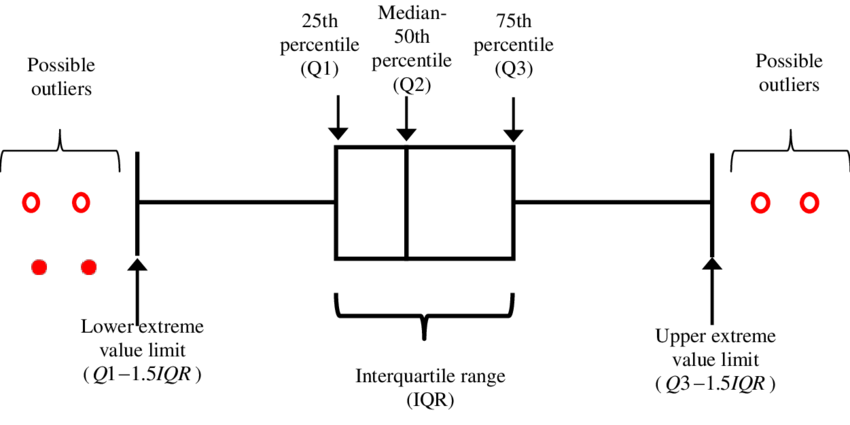
What is an outlier? How can outliers be determined in a dataset?

If you sort the salary data of 1000 employees in ascending order, then the salary information of the 250th person is 25th (Q1) percentile. Salary information of the 500th person is 50th (Q2) percentile. Salary information of the 750th person is 75th (Q3) percentile. The difference between Q3 and Q1 salary is called IQR (Interquartile Range). If you add 1.5IQR with Q3 you will get a salary, say 1.8 Lakh. Any salary more than this is considered a right side outlier. If you subtract 1.5IQR from Q1 then you will get a number, say 40K. Any salary less than this will be considered as a left side outlier.

What are the applications of outlier detection?

• Fraud detection in financial transactions
• Intrusion detection in infrastructure management
• Fault detection in manufacturing processes
• Data-preprocessing to remove anomalies in the dataset so that we can make a stable model.

How to handle missing data in a given dataset?

• Predict the missing values using other columns.
• Assignment of individual (unique) values. Let’s say city information is missing, you can say city1, city2 etc.
• Deletion of rows, which have the missing data. Deletion of column which has missing data.
• Mean imputation
• Median imputation
• Mode imputation
• Use other columns for Mean, Median, Mode imputation.

In statistics, what are the types of selection bias?

When you select some datapoint intentionally it is selection bias. You may not have the intention of introducing bias but because of your action it has come in the dataset. Following types of bias possible.

• Observer selection
• Attrition
• Protopathic bias
• Time intervals
• Sampling bias

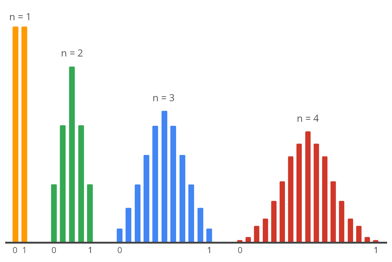
What is the central limit theorem (CLT)?

According to Central Limit Theorem

1. Population means can be known from sample mean. x̄ = μ + z * (σ / √n)

where:
x̄ (bar x) is the sample mean
μ is the population mean
z is the standard normal score (also known as a z-score)
σ is the population standard deviation
n is the sample size

The CLT states that as the sample size (n) increases, the sampling distribution of the mean (x̄) becomes more normal, and the sample mean becomes a more accurate estimate of the population mean (μ).

1. The standard deviation of the sampling distribution of the mean = SE = Sample’s SD = (σ/√n).

2. \(z = \frac{\bar{x}-\mu}{SE}, \qquad where \qquad SE = \frac{s}{\sqrt{n}}\) where \bar{x} is sample mean, s is sample SD

Can you explain what is the distribution in statistics, what purpose they serve?

There are two kinds of variables: numerical and categorical. Numerical variables like age of human, age of star, waiting time at service counter, growth of virus, distance between stars etc follows different types of continuous distributions. Discrete variables like city, color, education, pincode, plant name, building type, builder etc follow discrete distribution.

Common Distribution types are

• Continuous Distributions
  • Normal Distribution
  • Uniform Distribution
  • Cauchy Distribution
  • t Distribution
  • F Distribution
  • Chi-Square Distribution
  • Exponential Distribution
  • Weibull Distribution
  • Lognormal Distribution
  • Birnbaum-Saunders (Fatigue Life) Distribution
  • Gamma Distribution
  • Double Exponential Distribution
  • Power Normal Distribution
  • Power Lognormal Distribution
  • Tukey-Lambda Distribution
  • Extreme Value Type 1 Distribution
  • Extreme Value Type I Distribution
  • Beta Distribution
• Discrete Distributions
  • Binomial Distribution
  • Poisson Distribution

There are many kinds of distribution and each distribution has its related function. Some of the important functions related to each distribution are as below. Formulas for each function are different for different distribution types.

• Probability Density Function (pdf): PDF gives the probability that of variable at value x, e.g: pdf can give probability of variable (age) at value (=35 years)
• Cumulative Distribution Function (CDF): CDF is the probability that the variable takes a value less than or equal to x, e.g. CDF can give probability of variable (age) at value (<>=35 years)
• Percent Point Function (ppf) : It is Inverse of Distribution function (idf)
• Survival Function : The survival function is the probability that the variate takes a value greater than x, e.g. sf can give probability of variable (age) at value (>35 years)
• Inverse Survival Function: It is the Inverse of Survival function.
• Hazard Function: The hazard function is the ratio of the probability density function to the survival function, S(x).
• Cumulative Hazard Function: The cumulative hazard function is the integral of the hazard function.

Note: Each distribution has its own shape and measure to summarize the data. They are broadly of three types, measure of central tendency, measure of dispersion and shape of distribution. Following are common measures for every distribution. For example, to calculate central tendencies like mean, median of normal distribution there is some formula. In the case of exponential distribution central tendencies will not be arithmetic mean but geometric mean.

• Mean, Median, Mode, Range, SD, Kurtosis, Coefficient of Variation, SD, Skewness
• Each measure has different formula for calculation

Some Additional Notes for Data Scientists.

A data scientist is dealing with different streams of subjects like statistics, database, software engineering, geometry, vector and metrics, and calculus at the same time. There are certain terms which are referred to differently by different subjects. To avoid the confusion I am putting them below.

• Variable of statistics = Column of database = Field of database = Basis vector of geometry. They all refer to the same thing.
• Records of database = tuple of database = observation of statistics = vector of geometry.
• Slope of Geometry = Gradient of calculus = Gradient in Deep Learning and Machine Learning. The value of slope or gradient can be between \(-\infty \,\, to \,\,+\infty\)

Resources

• Statistics_Cartoon_Guide-BOOK
• Probability and Statistics for Data Science-BOOK
• Comprehensive & Practical Inferential Statistics Guide-GUIDE
• Statistics and Machine Learning in Python-BOOK
• Introduction to Probability and Statistics for Engineers and Scientists-BOOK
• Probability & Statistics with Applications to Computing-BOOK
• Statistics Demystified-BOOK
• HypothesisTesting-PPT
• What is a z-score? What is a p-value?

YouTube Resource for Statistical Test

• Choosing which statistical test to use - 10 min video
• Choosing a statistical test for analysis of data - 25 min video
• T test, Z test, F test, Chi-square test, ANOVA, Mann-Whitney U Test, H test - 33min video
• Two-sample t test for difference of means

Conclusion

Statistics is a big and complex subject and this is the foundational stone of any data science work, primarily for data analysis and model building. You may not be an expert in this subject and it can take a significant amount of time to get mastery over this subject. But with the help of the above questions a company can evaluate whether you are comfortable enough in the subject to take challenges in a data science project. If you would like to add your favorite questions then you can email me at hari.prasad@vedavit-ps.com