
Timeseries Interview Questions#
What are the characterstics of time series data?#
Time series data is a series of data points collected over time. Some characteristics of time series data include:
- Time dependence: Time series data is typically collected at regular time intervals, and the values of the time series are often dependent on the time at which they were collected.
- Equal duration gap between samples/ records
- No missing record in between
- Trend: Many time series exhibit a long-term trend, either upward or downward. This trend may be influenced by a variety of factors such as economic conditions, population growth, or technological changes.
- Seasonality: Many time series exhibit regular fluctuations due to seasonal factors such as weather, holidays, or other events. For example, retail sales may be higher in the months leading up to Christmas due to holiday shopping.
- Cyclicity: Time series may exhibit cyclical pattern. Like sales is highest in month start, body temprature is high at 6am, traffic is least on weekends etc.
- Noise: Time series data may also be affected by random noise or error, which can make it difficult to accurately forecast future values.
- Autocorrelation: Time series data may exhibit autocorrelation, which is the phenomenon of a value at a particular time being correlated with values at nearby times. This can make it challenging to model the time series, as the value at a given time may depend on the values at nearby times.
Example of time series data#
| Date | Sales (y) |
|---|---|
| 2020-01-01 | 1000 |
| 2020-02-01 | 1100 |
| 2020-03-01 | 1200 |
| 2020-04-01 | 1100 |
| 2020-05-01 | 1000 |
| 2020-06-01 | 900 |
| 2020-07-01 | 1200 |
| 2020-08-01 | 1400 |
| 2020-09-01 | 1300 |
| 2020-10-01 | 1500 |
This first column can be date or date or datetime. Interval between two rows must be equal. The unit of date or time or datetime may be milliosecond, or second, or minute, or hour, or day, week, month, quarter, year or dacade. This should be continuous without any gap.
Second column can be any measurment like sales, temprature, purchase, railfall, production, infections, number of infections, etc.
What is the difference between noise and stationarity?#
Noise and stationarity are two different concepts in time series analysis.
Noise refers to random fluctuations in a time series data that do not follow a specific pattern. Noise can be caused by various factors such as measurement errors, random variations in the data, or external factors that are not related to the underlying process being measured. Noise can make it difficult to identify patterns and trends in the data, and can also cause problems when trying to make predictions based on the data.
Stationarity, on the other hand, refers to the property of a time series data where the statistical properties (such as mean and variance) do not change over time. A stationary time series is one that has a constant mean and variance over time, and is characterized by the presence of random fluctuations around the mean. Stationary time series are easier to model and predict because the statistical properties of the data do not change over time.
What do you mean by statistical properties#
Various statistical properties of data include the mean, median, mode, standard deviation, variance, skewness, kurtosis, correlation coefficient, coefficient of determination, and regression analysis. These properties are used to describe, analyze, and interpret quantitative data. They can also be used to make predictions and draw conclusions about data.
What are the assumptions of a stationary time series?#
A stationary time series is a time series that has constant statistical properties over time. In other words, the mean, variance, and autocovariance of the time series do not depend on the time index.
There are several assumptions that are typically made about stationary time series:
- The mean of the time series is constant over time.
- The variance of the time series is constant over time. (Don’t confuse this is zero variance)
- The autocovariance of the time series depends only on the time lag between observations, and not on the time at which the observations are made.
- A time series is “weakly stationary,” meaning that the statistical properties of the time series are unchanged under time shifts.
It is important to check for stationarity before performing certain types of time series analysis, as many time series models and techniques are based on the assumption of stationarity.
What is a Statitionary Time Series#
A stationary time series is a time series that has constant statistical properties over time. In other words, the mean, variance, and autocovariance of the time series do not depend on the time index.
A stationary time series is said to be “strictly stationary” if the statistical properties of the time series are completely constant over time. This means that the mean, variance, and autocovariance of the time series are all constant.
A stationary time series is said to be “weakly stationary” if the statistical properties of the time series are unchanged under time shifts. This means that the mean, variance, and autocovariance of the time series are all constant, but the time series may have a non-zero mean.
It is important to check for stationarity before performing certain types of time series analysis, as many time series models and techniques are based on the assumption of stationarity.
What is the difference between variance, covariance and autocovariance?#
Variance, covariance, and autocovariance are all measures of the dispersion of a set of data. However, they are used to measure different types of dispersion.
- Variance: Variance is a measure of the dispersion of a single set of data. It is calculated as the sum of the squared differences between each data point and the mean of the data, divided by the number of data points. For example variance of age data.
- Covariance: Covariance is a measure of the dispersion of two sets of data. It is calculated as the sum of the products of the differences between each data point in one set and the mean of that set, and the differences between the corresponding data points in the other set and the mean of that set, divided by the number of data points. Covariance can be used to determine the relationship between two sets of data. For example, covariance between age and experience.
- Autocovariance: Autocovariance is a measure of the dispersion of a single time series at different time lags. It is calculated as the covariance between observations at time $t$ and observations at time $t+k$, where $k$ is the time lag between the observations. Autocovariance can be used to determine the relationship between observations in a time series at different points in time. For example, autocovarince of sales date at monthly interval.
What is Additive Model in time series?#
In a time series, an additive model is one where the overall effect of the various factors (such as trend, seasonality, and noise) is simply the sum of their individual effects.
For example, if we have a time series that is influenced by trend, seasonality, and noise, an additive model would express the time series as:
y(t) = trend(t) + seasonality(t) + noise(t)
where y(t) is the value of the time series at time t, trend(t) is the trend component at time t, seasonality(t) is the seasonality component at time t, and noise(t) is the noise or error component at time t.
In an additive model, the individual components can be estimated independently and then summed to produce a model for the time series. This can make it relatively simple to build and interpret the model, especially if the individual components are easy to identify and separate. However, additive models may not always be the best choice, especially if the various factors are not truly independent or if the relationship between the time series and the factors is more complex than a simple sum.
Examples:
- Monthly sales of a retail store
- Quarterly earnings of a public company
- Daily temperature in a particular city
- Hourly traffic on a specific stretch of road
- Monthly unemployment rate in a country
What is multiplicative Model in time series?#
In a time series, a multiplicative model is one where the overall effect of the various factors (such as trend, seasonality, and noise) is the product of their individual effects.
For example, if we have a time series that is influenced by trend, seasonality, and noise, a multiplicative model would express the time series as:
y(t) = trend(t) _ seasonality(t) _ noise(t)
where y(t) is the value of the time series at time t, trend(t) is the trend component at time t, seasonality(t) is the seasonality component at time t, and noise(t) is the noise or error component at time t.
In a multiplicative model, the individual components can be estimated independently and then multiplied to produce a model for the time series. This can be a useful approach if the time series exhibits exponential growth or decay, or if the relationship between the time series and the various factors is more complex than a simple sum. However, multiplicative models may be more difficult to interpret than additive models, and they may not always be the best choice, especially if the various factors are not truly independent.
Examples
- Daily stock price of a public company
- Annual population growth rate of a country
- Monthly revenue of a subscription-based business
- Virus growth
- Weekly sales of a product with a limited lifespan (such as a food product with a short shelf life)
What are the test of Stationarity#
A stationary time series is one whose statistical properties (such as the mean, variance, and autocorrelation) are constant over time. Stationarity is an important assumption for many time series analysis techniques, as it implies that the statistical properties of the time series do not change over time. This makes it easier to model the time series and make forecasts about future values.
There are several tests that can be used to determine whether a time series is stationary or not. Some common tests include:
- Augmented Dickey-Fuller (ADF) test: This test looks at the difference between the time series and a lagged version of itself to determine whether the time series is stationary.
- Kwiatkowski-Phillips-Schmidt-Shin (KPSS) test: This test looks at the level of trend and seasonality in the time series to determine whether it is stationary.
- Philips-Perron (PP) test: This test is similar to the ADF test, but it is more robust to the presence of autocorrelation in the time series.
- Median absolute deviation (MAD) test: This test looks at the dispersion of the time series around its median value to determine whether it is stationary.
It’s worth noting that these tests are statistical in nature, and they can only provide a certain level of confidence in whether a time series is stationary or not. In some cases, further analysis may be needed to determine whether a time series is truly stationary.
How regression is different from correlation?#
In regression we predict a number (dependent variable) with the help of predictor (independent variables) $$ y = \beta_0 + \beta_1*x$$
In correlation we check degeree and magnitude of relationship between two variables. It’s value can be between -1 to +1. 0 Means there is no relationship. There are several statistical tests that can be used to measure the correlation between two variables. Some common tests include:
Pearson’s correlation coefficient: This is the most well-known measure of correlation, and it measures the linear relationship between two variables. The Pearson correlation coefficient is calculated as: $$ \rho_{(x,y)} = \frac { Cov(x, y)} {(Std(x) * Std(y)) }$$
Spearman’s rank correlation coefficient: This measure of correlation is based on the ranks of the data rather than the raw data values, and it can be used to measure the strength of a monotonic relationship between two variables. The Spearman rank correlation coefficient is calculated as: $$ \rho_{(x,y)} = 1 - \frac {6 ∑d^2} {n(n^2 - 1)}$$
where d is the difference in ranks between the two variables, and n is the number of data points.
Kendall’s tau: This measure of correlation is similar to the Spearman rank correlation coefficient, but it is based on the number of concordant and discordant pairs of data rather than the ranks of the data. The Kendall tau correlation coefficient is calculated as: $$ \tau = \frac {(c - d)} { \sqrt(c + d)}$$
where c is the number of concordant pairs and d is the number of discordant pairs.
It’s worth noting that these correlation tests are statistical in nature, and they can only provide a certain level of confidence in the strength of the relationship between two variables. In some cases, further analysis may be needed to fully understand the nature of the relationship.
What is Autoregression (AR) Model?#
When we can predict value at k time period from the value available at time t. If we can predict sales for next week (k=7 days ahead) from the sales of today (t) then this autoregression.
Autoregression (AR) is a statistical model that describes a time series as a linear function of its own past values. For example, an autoregressive model of order 1 (AR(1)) can be written as:
y(t) = c + φ1*y(t-1) + ε(t)
where y(t) is the value of the time series at time t, c is a constant, φ1 is the autoregressive coefficient, y(t-1) is the value of the time series at the previous time step (t-1), and ε(t) is the error term.
What is Autocorrelation?#
Autocorrelation (also known as serial correlation or lagged correlation) is the statistical dependence between a time series and a lagged version of itself. For example, the autocorrelation between a time series y(t) and a lagged version of itself y(t-k) can be measured using the Pearson correlation coefficient:
When value at t time period has some relationship with a value at t+k time then we say there is autocorrelation. Like coorelation value of this can be between -1 to 1.
What is the importance of ACF and PACF plots#
Autocorrelation function (ACF) and partial autocorrelation function (PACF) plots are graphical tools used to examine the autocorrelation of a time series.
ACF plots show the autocorrelation of a time series with itself at different lag values. For example, an ACF plot for a time series y(t) might show the autocorrelation between y(t) and y(t-1), y(t) and y(t-2), and so on. The ACF plot can help identify patterns in the autocorrelation of the time series, such as whether the autocorrelation decays exponentially or exhibits a more complex pattern.
PACF plots show the partial autocorrelation of a time series with itself at different lag values. Partial autocorrelation measures the correlation between a time series and a lagged version of itself, controlling for the effects of all other lagged values. The PACF plot can help identify the number of autoregressive (AR) terms that are needed to model the time series.
ACF and PACF plots are useful tools for understanding the autocorrelation structure of a time series, and they can help inform the choice of statistical models and forecasting methods. For example, if the ACF plot of a time series exhibits a strong decay at a particular lag value, an autoregressive model with a single lag (AR(1)) may be sufficient to model the time series. On the other hand, if the ACF plot exhibits a more complex pattern, a higher-order autoregressive model (such as AR(2) or AR(3)) may be needed.
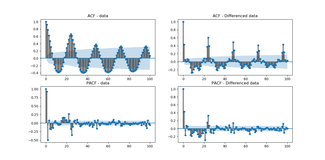
Estimating AR terms The lollipop plot that you see above is the ACF and PACF results. To estimate the amount of AR terms, you need to look at the PACF plot. First, ignore the value at lag 0. It will always show a perfect correlation, since we are estimating the correlation between today’s value with itself. Note that there is a blue area in the plot, representing the confidence interval. To estimate how much AR terms you should use, start counting how many “lollipop” are above or below the confidence interval before the next one enter the blue area.
So, looking at the PACF plot above, we can estimate to use 3 AR terms for our model, since lag 1, 2 and 3 are out of the confidence interval, and lag 4 is in the blue area.
What are different smoothing techniques for timeseries data?#
There are several smoothing techniques that can be used for time series data. Some common techniques include:
Moving average: This method involves replacing each data point with the average of a certain number of preceding and following points. This can help to smooth out short-term fluctuations and highlight longer-term trends.
Exponential smoothing: This method assigns a higher weight to more recent observations and a lower weight to older observations. This can help the model to better capture the underlying trend in the data.
Lowess: This method fits a smooth curve to the data using locally weighted linear regression. It can effectively smooth out noise and highlight the underlying trend in the data.
Seasonal decomposition: This method involves separating the data into three components: trend, seasonality, and residual. The trend component can then be smoothed to better understand the long-term behavior of the data.
Savitzky-Golay filter: This method fits a polynomial to a window of data points and then uses the polynomial to predict the value of the center point in the window. This can help to smooth out short-term fluctuations while preserving important features in the data.
What is Maximum Likelihood Expectation (MLE), how to calculate MLE?#
The “likelihood function” is used to estimate the parameters of a model that best fit the data. Given a set of parameters for a statistical model, “Likelihood Function” is a function that describes the probability of obtaining a set of observations.
θ for ARIMA model is values of p,d,q parameters which we want to know. The meaning of L(θ;x) function is given x (data) what is the value of likelihood with different parameters values or different θ(p,d,q).
The “maximum likelihood estimation” (MLE) is a method to find the set of parameters that maximize the likelihood function. The MLE method searches for the set of parameters that makes the observed data most probable. In other words, it maximizes the likelihood function.
maximum likelihood estimation (MLE) method is given by:
$$\hat{\theta} = argmax_{\theta} L(\theta;x)$$
Means maximum values of θ(p,d,q) parameters for the given data.
Where:
$$\hat{\theta}$$ is the maximum likelihood estimate of the parameter vector $$\theta$$ is the parameter vector $$L(\theta;x)$$ is the likelihood function, which is a function of the parameters and the data $$x$$ is the data The likelihood function is typically defined as the product of the probability densities of the observations, given the parameters of the model:
$$L(\theta;x) = f(x|\theta) = \prod_{i=1}^{n} f(x_i|\theta)$$
where:
$$f(x_i|\theta)$$ is the probability density function of the i-th observation given the parameters $$n$$ is the number of observations Note that logarithm of the likelihood function is taken in practice as the product of large number of small numbers can cause floating point underflow.
$$log (L(\theta;x)) = log(\prod_{i=1}^{n} f(x_i|\theta)) = \sum_{i=1}^{n} log(f(x_i|\theta))$$
And then maximizing the logarithm of the likelihood function is the same as maximizing the likelihood function.
Let’s say we have a time series data of profit for a retail store, and we want to fit one ARIMA model to it. The likelihood function for the ARIMA model would be a function of the parameters of the model (p,d,q) and the data.
To find the maximum likelihood estimation of the parameter θ, we would need to differentiate the likelihood function with respect to θ and set it equal to zero. Then, we would solve for the value of θ that maximizes the likelihood function.
∂L/∂θ = 0
Solving for θ, we get the maximum likelihood estimate for the parameter.
“L” is the maximum value of the likelihood function for the model, which is the probability of obtaining the observed data given the parameters of the model.
ARIMA(1,0,0) likelihood function: $$L = (2πσ^2)^{-n/2} e^{-\frac{1}{2σ^2}\sum_{t=2}^n(y_t - μ - φ(y_{t-1} - μ))^2}$$
ARIMA(1,1,1) likelihood function: $$L = (2πσ^2)^{-n/2} e^{-\frac{1}{2σ^2}\sum_{t=2}^n(y_t - μ - φ(y_{t-1} - μ) - \theta(y_{t-1} - y_{t-2} - μ))^2}$$
ARIMA(1,2,1) likelihood function: $$L = (2πσ^2)^{-n/2} e^{-\frac{1}{2σ^2}\sum_{t=3}^n(y_t - μ - φ(y_{t-1} - μ) - \theta(y_{t-1} - 2*y_{t-2}+y_{t-3} - μ))^2}$$
ARIMA(2,2,2) likelihood function: $$L = (2πσ^2)^{-n/2} e^{-\frac{1}{2σ^2}\sum_{t=3}^n(y_t - μ - φ_1(y_{t-1} - μ) - \phi_2(y_{t-2} - μ) - \theta_1(y_{t-1} - y_{t-2} - μ) - \theta_2(y_{t-2} - y_{t-3} - μ))^2}$$
ARIMA(1,2,3) likelihood function: $$L = (2πσ^2)^{-n/2} e^{-\frac{1}{2σ^2}\sum_{t=4}^n(y_t - μ - φ(y_{t-1} - μ) - \theta_1(y_{t-1} - 2y_{t-2}+y_{t-3} - μ) - \theta_2(y_{t-2} - 3y_{t-3}+3y_{t-4}-y_{t-5} - μ) - \theta_3(y_{t-3} - 4y_{t-4}+6y_{t-5}-4y_{t-6}+y_{t-7} - μ))^2}$$
where y(t) is the observed data, μ is the mean of the data, σ^2 is the variance of the data, n is the number of observations, and φ is the parameter of the model.
What is AIC, BIC?#
AIC (Akaike Information Criterion) and BIC (Bayesian Information Criterion) are both measures of the relative quality of statistical models. They are used to compare different models and select the one that best fits the data.
AIC is defined as:
AIC = 2k - 2ln(L)
where k is the number of parameters in the model and L is the maximum value of the likelihood function for the model. AIC is a measure of the relative quality of a statistical model, with lower values of AIC indicating a better model. It is used to compare different models and select the one that best fits the data.
BIC function is defined as:
BIC = kln(n) - 2ln(L)
where k is the number of parameters in the model, n is the number of observations and L is the maximum value of the likelihood function for the model. BIC is also a measure of the relative quality of a statistical model, with lower values of BIC indicating a better model. It is used to compare different models and select the one that best fits the data.
For example, let’s say we have two models, Model A and Model B, that we want to compare. Model A has 5 parameters and Model B has 10 parameters. We can use AIC or BIC to determine which model is the better fit for the data.
Let’s say, the AIC and BIC values for Model A are 100 and 150 respectively, and the AIC and BIC values for Model B are 150 and 200 respectively.
In this case, Model A would be a better fit for the data as it has lower AIC and BIC values than Model B.
It’s worth noting that AIC and BIC are based on different assumptions and have different properties, AIC is known to be less conservative than BIC, and it tends to favor models with more parameters. On the other hand, BIC is more conservative and tends to favor models with fewer parameters, which is more suitable for cases where the sample size is large.
What is ARIMA#
ARIMA (AutoRegressive Integrated Moving Average) is a statistical method for time series forecasting. It is a combination of three components:
AutoRegression (AR): The AR component represents the relationship between an observation and a number of lagged observations. It models the dependence between an observation and a number of lagged observations of the same variable. For example at lag 1, AR is .5, and at lag=2 AR is .6, at lag=3 AR is .7 etc.
Integration (I): The I component represents the difference between the raw observation and the observation after being differenced. It is used to make the time series stationary. For example at lag=3 where AR is highest we take difference between acutual observation and lagged observation and get the difference for all the observations. This is called error.
Moving Average (MA): The MA component represents the relationship between the observation and the error term. It models the dependence between an observation and a moving average of error terms. For example we take MA for above error terms when we average 2 observation, or we can take MA 3 observation or 4 observation. We do this for all the observation.
ARIMA models are used to predict future values of a time series based on its past values and the error term. The model is trained on historical data and is then used to make predictions on new data. The model parameters are chosen through a process called model selection which involves estimating the model parameters using statistical methods and selecting the best set of parameters based on some criteria like AIC, BIC.
ARIMA models are used in timeseries forecasting, and are particularly useful for modeling and forecasting time series with a seasonal component.
What is ARIMAX#
What is SARIMAX model?#
SARIMA stands for Seasonal Autoregressive Integrated Moving Average. It incorporates the seasonal component in addition to the autoregressive and moving average components that are present in the basic ARIMA model. The SARIMA model also includes a seasonal differencing component, which is used to account for the repeating patterns in the data that occur at regular intervals (e.g. monthly or quarterly data). The model is specified using three parameters: (p,d,q) for the autoregressive component, (P,D,Q) for the seasonal component, and m for the number of seasons. The notation SARIMA(p,d,q)(P,D,Q)m is used to represent a SARIMA model.
What is the difference between white noise and a stationary time series.#
What are some common drawbacks of the ARIMA set of methods? What are the different ways to overcome them?#
Explain the importance of parameter choosing for every technique in smoothing methods and the ARIMA set of methods and how they can choose the best working parameter.#
What are the common mistakes people make while using the ARIMA set of methods?#
How to identify the best working model for time series analysis.#
Important Libraries for Timeseries Model Building#
Common Libraries supporting Timeseries model or visulzation or task#
- Numpy
- Pandas
- Matplotlib
- Seaborn
- Scikit-learn
- TensorFlow
- Keras
- PyTorch
- XGBoost
- LightGBM
- CatBoost
Libraries supporting Timeseries model#
- sktime
- Prophet
- Statsmodels
- Fbprophet
- GluonTS
- TimeSeriesNet
- LSTNet
- DeepST
- tsfresh
- pmdarima
- minisom
Libraries Supporting Timeseries Other Work#
- TimeSeriesSplit
- TimeSeriesGenerator
- TimeSeriesForecast
- TimeSeriesAnalysis
- TimeSeriesClustering
- TimeSeriesClassification
- TimeSeriesRegression
- TimeSeriesDeepLearning
- TimeSeriesNLP
What are different types of timeseries data?#
There are several types of time series data, including:
- Univariate time series: This type of data consists of a single variable measured over time. Examples include stock prices, temperature, and rainfall.
- Multivariate time series: This type of data consists of multiple variables measured over time. Examples include weather data with multiple variables such as temperature, humidity, and wind speed.
- Panel data: Also known as cross-sectional time series data, this type of data consists of multiple observations of multiple variables over time. Examples include data on individuals, households, or firms, collected at different time points.
- Hierarchical time series: This type of data consists of multiple levels of observations, such as data collected at different geographic locations or different subpopulations.
- Spatial-temporal data: This type of data consists of observations of variables at different locations and times. Examples include data on air pollution or crime rates.
- Time series with exogenous variables: This type of data includes additional variables that are not measured over time, but may influence the time series.
- Irregular time series: This type of data has observations that are not evenly spaced in time, such as data collected at irregular intervals or with missing observations.
- Time series with trend: This type of data has a long term upward or downward trend, which can make it difficult to predict future values.
- Cyclical time series: This type of data has repeating patterns, such as seasonal data with a regular pattern of ups and downs.
- Stochastic time series: This type of data has random fluctuations that are not explained by any underlying patterns or trends.
- Time series with seasonality: This type of data has regular patterns that repeat over a specific period of time, such as daily, weekly, or yearly. For example, retail sales tend to be higher during holidays, or energy consumption tends to be higher during weekdays than weekends.
- Time series with multiple seasonality: This type of data has more than one seasonality, such as daily and weekly patterns.
- Non-stationary time series: This type of data has a mean or variance that changes over time, making it difficult to predict future values.
- Stationary time series: This type of data has a constant mean and variance over time, and is characterized by the presence of random fluctuations around the mean.
- Cointegrated time series: This type of data has two or more time series that have a long-term relationship, such as stock prices and interest rates.
- Causal time series: This type of data is affected by one or more external variables, known as explanatory or predictor variables, that can be used to predict future values.
- Non-causal time series: This type of data is not affected by any external variables, and can only be predicted using past values of the same time series.
- Event-based time series: This type of data is affected by specific events, such as product launches, natural disasters, or political changes.
These time series types can also be combined in certain scenarios. They are not mutually exclusive.

Comments: